(Before starting I will say that this post, as the whole blog, is speculative and heterodox. I wanted to say it for the case that someone arrives here looking for info to study these subjects. The purpose of this blog is to think and to inspire others, not to teach them. I propose you to start thinking by yourself and to read everything in a critic way).
As you will know, one of the so-called «millennium problems» is the «Hodge Conjecture».
The Clay Institute’s website http://www.claymath.org/millennium-problems/hodge-conjecture tells us that «In the twentieth-century mathematicians discovered powerful ways to investigate the shapes of complicated objects. The basic idea is to ask to what extent we can approximate the shape of a given object by gluing together simple geometric building blocks of increasing dimension.».
(So, it comes to using simple geometric pieces of an increasing size to create a figure that is as similar as possible to the shape of a complicated figure. The use of infinite or infinitesimal approximations to a curved shape by using a straight line or a quadratic figure is what already Newton and Leibniz did in the XVII century giving rise the so-called integral and differential calculus).
The presentation continues saying that «This technique turned out to be so useful that it got generalized in many different ways, eventually leading to powerful tools that enabled mathematicians to make great progress in cataloging the variety of objects they encountered in their investigations».
(When they speak about algebraic objects they are thinking about abstract “objects» on abstract «spaces»).
«Unfortunately, the geometric origins of the procedure became obscured in this generalization. In some sense, it was necessary to add pieces that did not have any geometric interpretation. The Hodge conjecture asserts that for particularly nice types of spaces called projective algebraic varieties, the pieces called Hodge cycles are actually (rational linear) combinations of geometric pieces called algebraic cycles».
This paragraph clearly recognizes the drama that is that mathematicians have developed algebraically in a so abstract way geometric structures whose geometry is actually unknown for them. In many cases, it does not implies a problem for mathematicians who are very used to working with abstractions, but at least when it comes to Hodge cycles that total abstraction is the main problem to understanding and solving the Hodge conjecture.
The mentioned paragraph tries to explain the Hodge conjecture in an accessible way but, at first sight, it’s totally unintelligible for every persona who did not study mathematics (and maybe for many people who did it) because, outside of algebra, what are projective algebraic varieties and algebraic cycles? Without understanding these technic terms we won’t be able to understand, even in a general way, the problem that the Hodge conjecture is about.
People who do not understand algebra need to see a visual representation of those things they are working with to be able to understand them. But when it comes to Hodge cycles we already know that they are geometric pieces whose geometric representation is unknown. So its explanation outside algebra gets very difficult. (As I said before, it’s also very difficult inside of algebra itself because of the same reason, if the geometry of those Hodge pieces were clearly known the Hodge structures would naturally clarify the Hodge conjecture).
The geometric representation of algebraic cycles is known, though. So, we have actually some clues that we can follow almost as if we were detectives. A «cycle» is a geometric shape, and an “algebraic cycle» can be a curved shape intersected in several points by a straight line.
There is an explanation about the Hodge conjecture (to me it’s not very clear but it provides us some clues as this one about the visual algebraic cycles) made by an American professor of Austin University, Daniel Freed, where he shows some visual representations of algebraic cycles: https://www.ma.utexas.edu/users/dafr/HodgeConjecture/netscape_noframes.html
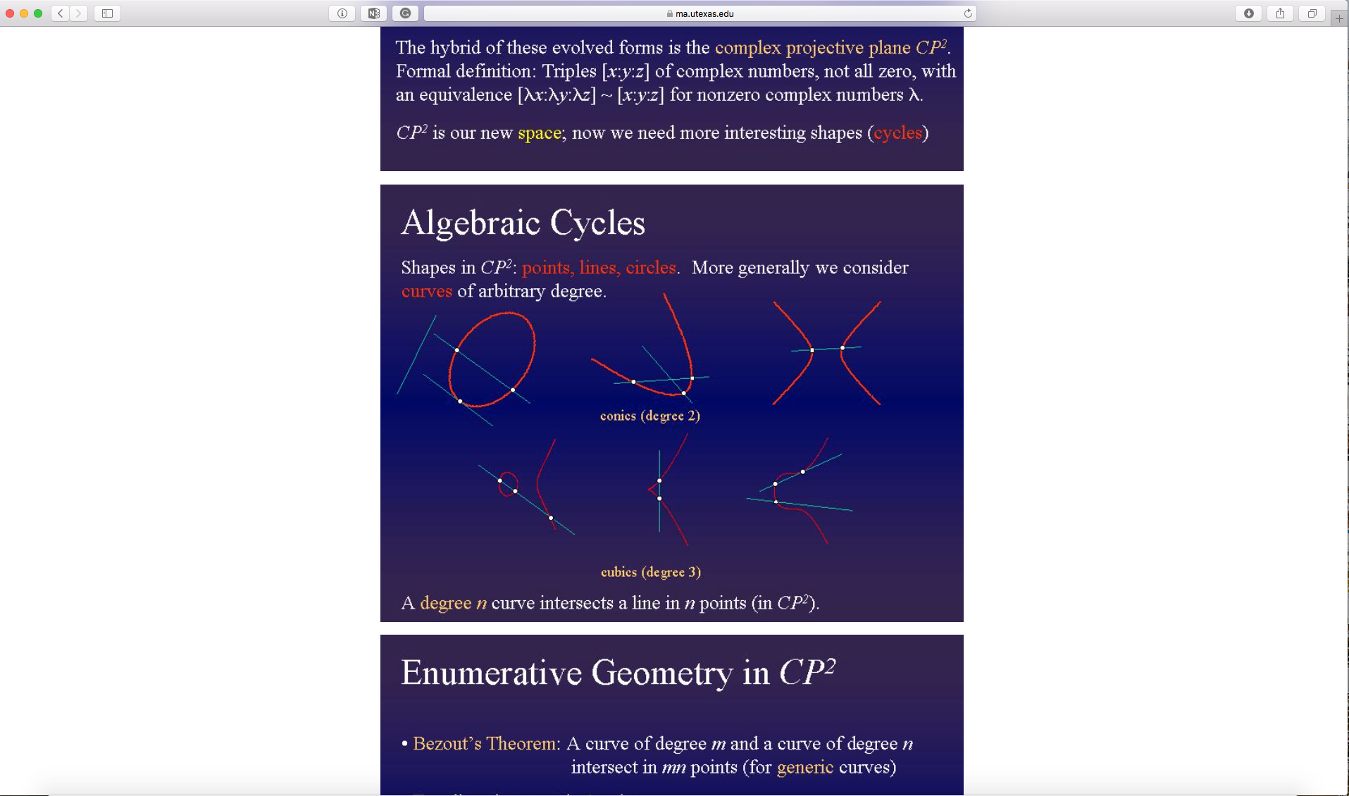
Then we can guess that the cycles related to the Hodge conjecture are combinations of these kind of curves.
We still need to understand in a visual way what a projective algebraic variety is, but we can suppose it’s about projecting (or prolonging) curves and that they create a smooth geometric space.
You can watch the professor Freed’s conference about the Hodge Conjecture here: http://claymath.msri.org/hodgeconjecture.mov
To me, none of the explanations I looked for in the internet about the Hodge Conjecture is actually understandable, except, this article written by a Spanish professor of the Complutense University of Madrid, Vicente Muñoz, who is a Hodge Theory’s specialist. It’s a divulgative article (he has at least another article that is much more technic) without using algebra:
https://ojs.uv.es/index.php/Metode/article/view/8253/10747
When I read the Clay Institute’s presentation about the Hodge Conjecture I had the feeling it was speaking, with different terms about something very similar to the so-called «Inverse Galois» problem and to the «Embedding problem» into a higher extension.
These are not considered millennium problems but they are issues related to the Galois theory that still are not solved.
I already spoke about Galois theory in previous posts (I think mainly in Spanish). You will know that the Galois theory appeared trying to explain why the equations of a degree higher than 4 are not solvable with simple mathematical operations (addition, subtraction, etc), as Neils Abel had already demonstrated some years before. Galois arrived to the conclusion that in the polynomial equations (i.e Xˆ5 + Xˆ4 + Xˆ3 + Xˆ2 + X = 0) there are symmetry groups and that when it comes to the 5th grade, the symmetry gets broken in such a way that is not possible to solve it in the same way we can solve lower degree equations, with simple mathematical operations.
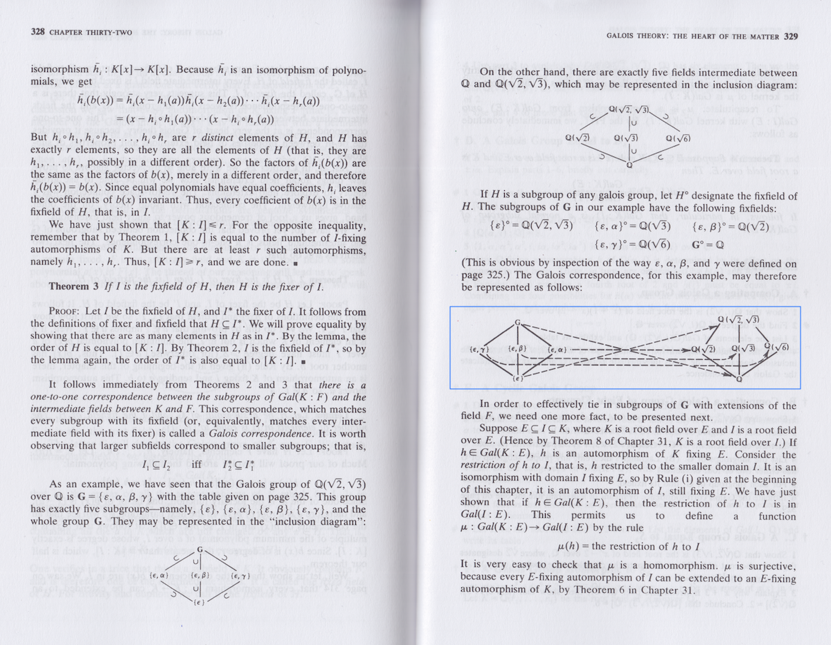
When it comes to Galois groups, the terminology that mathematicians use is «Field» (In French and in Spanish it has been translated as «body») that would be an initial or basic field, “Extension» (that is a field that contains inside a smaller field), subfields and subextensions, (intermediate extensions between an initial field and a given extension of it, or between a given extension and a given subextension of it).
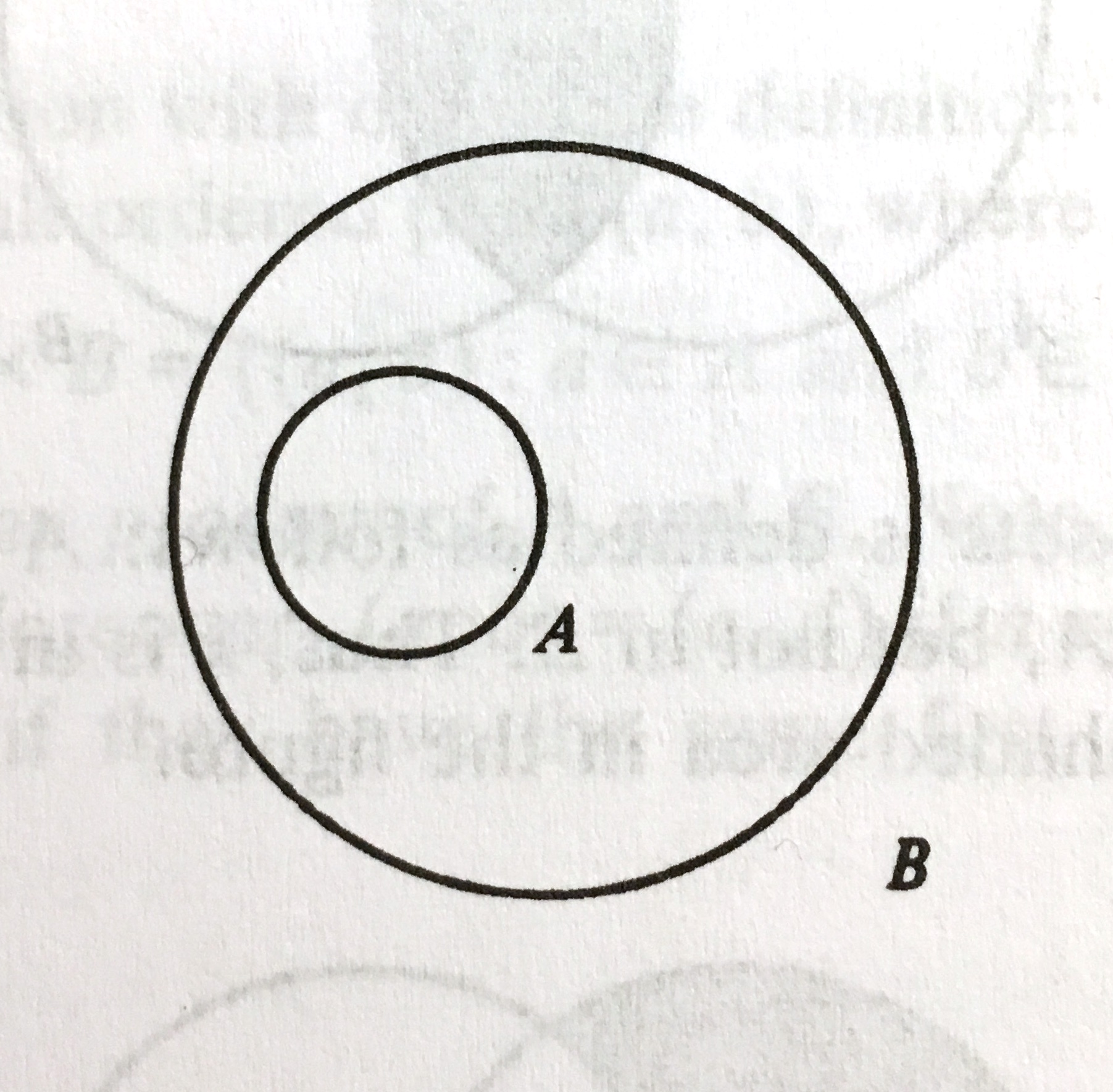
(In this picture B is an extension of A).
I mentioned in previous posts that I had sent to different people the diagrams I was doing asking them if they could be visual representations of Galois groups, fields and extensions. Also I asked it in some forums, and no one was able to confirm or to deny it. the Galois theory and all the Groups theory (and almost most of the mathematical developments of the last two centuries) had been made in a purely and exclusively abstract and algebraic way. There are not (or there are very few) visual representations of Galois groups.
But with those diagrams and only understanding some few concepts as what an extension is, it’s possible to follow explanations without algebra about Galois groups and to understand and to anticipate and to deduce technical concepts as isomorphism, homomorphism, automorphism, and to understand the immersion and the inverse Galois problems.
The inverse Galois problem can be explained in these terms: If we have a given extension of a given initial field, so we have a larger field that contains inside a smaller field, how can we know – or to build – what are the intermediate subextensions (that follow in a continuous way the same symmetric structure and keep the same initial and final image) between that larger extension and the smaller initial field.
I don’t know if this is a free interpretation I do about the Inverse problem but I understood it in this way.
And the «embedding» problem is actually the same but instead of considering it from outside to inside or from the end to the beginning, considering it from the beginning of an initial field to the end of a larger given extension. How can we build the intermediate subextensions where the initial field or another subextensions of that extension is embedding?
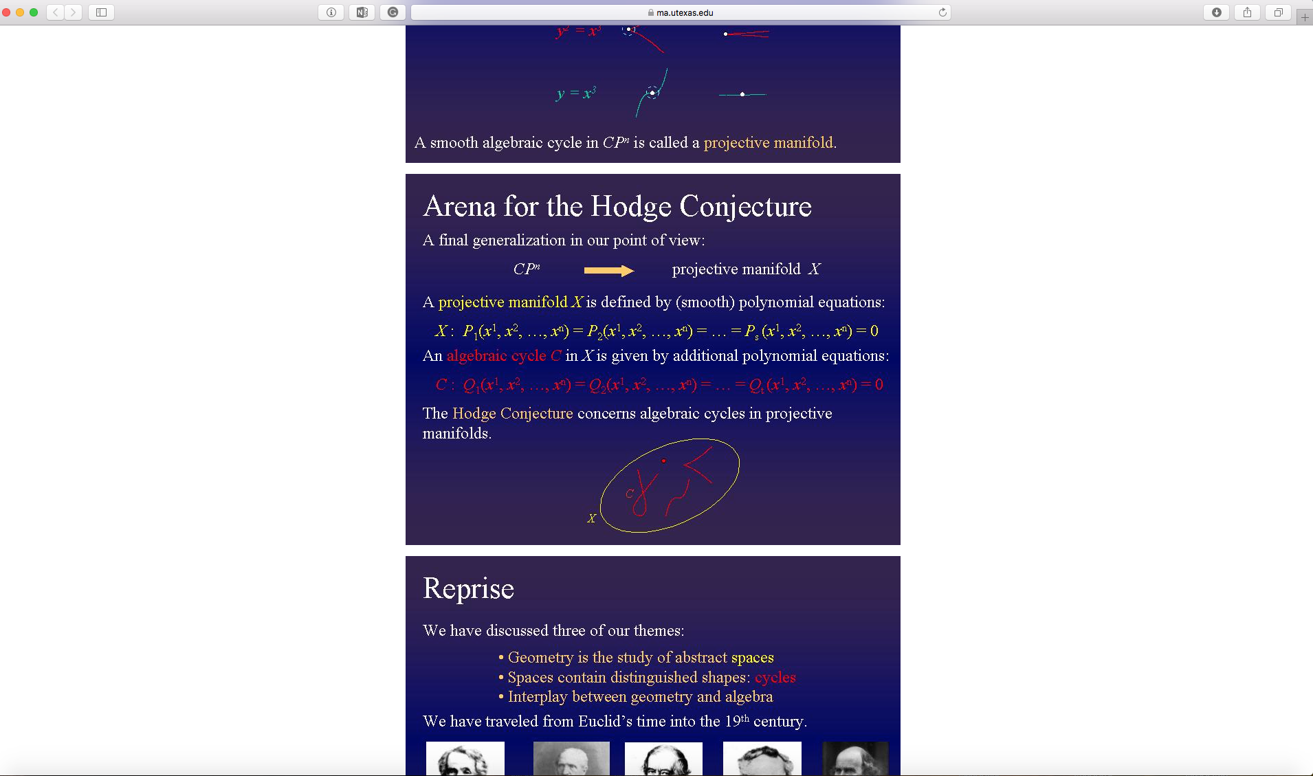
To me, the Hodge problem is also about the same issue: If we have a smooth structure on a space that we called projective algebraic variety created by projecting an initial field created by the opposite curves that we call algebraic cycles, how can we create that smooth structure by combining those algebraic cycles and their projections? (or how can know if that smooth structure is formed by existing combinations of those algebraic cycles and their projections?). Those combinations of the algebraic cycles and the projected algebraic cycles would be the hedge cycles or Hodge shapes.
I thought that if the Galois problem was the same or a similar one, there likely should be any clue about it in the mathematical literature, that mathematicians would become aware and have related those problems. In fact I found that the so-called Tate Conjecture» that is the arithmetic version of the Hodge Conjecture describe the algebraic cycles of a variety in terms of the Galois representation they call étale cohomology: https://en.wikipedia.org/wiki/Tate_conjecture
One of the issues I discuss with some about the posts I wrote related to Galois theory was that solvability of quintic equations
If the Galois theory tells us that we cannot solve the quintic or higher equations because of the symmetry of the groups gets broken beyond the fourth degree, how it is possible the symmetry is kept for any degree in the polynomials I’m representing in the mentioned diagrams. If the symmetry is preserved, why the quintic and higher equations could not be solved with simple mathematical operations? Maybe they were not Galois fields and extensions? I arrived to the conclusion that the Galois theory uses a unique polynomial equation (Xˆ1 + Xˆ2 + Xˆ3 + Xˆ4 + X^5) while I was combining the elements of different polynomial equations P1 (Xˆ1 + Xˆ2 + Xˆ3 + Xˆ4 + X^5), P2 (Xˆ1 + Xˆ2 + Xˆ3 + Xˆ4 + X^5), P3 (Xˆ1 + Xˆ2 + Xˆ3 + Xˆ4 + X^5), P4 (Xˆ1 + Xˆ2 + Xˆ3 + Xˆ4 + X^5), P5 ((Xˆ1 + Xˆ2 + Xˆ3 + Xˆ4 + X^5).
Something similar appears in the prof. Freed’s conference when speaking about the Hodge conjecture arena:
To this respect also it is revealing what the professor Muñoz, in his divulgative work about the Hodge conjecture mentions that «The Hodge conjecture is difficult because complex manifolds are very rigid objects (since they are defined by polynomials). In fact is very difficult to construct complex manifolds and there are very few of them. Proving that submanifolds exist without constructing them has also been difficult».
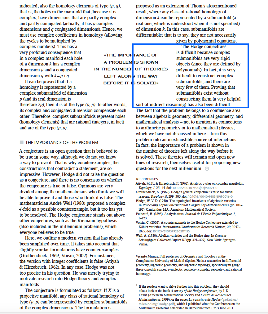
To me, that statement is very weird because polynomials are not rigid structures since the moment they can be combined. Combination is actually what the Hodge cycles consist about. But it’s extremely difficult being aware of it working from an abstract algebraic or even arithmetic perspective without having any visual references.
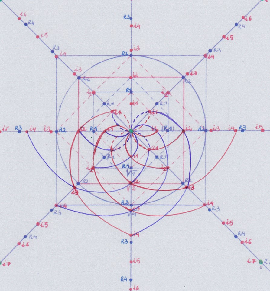
So, now I’m going to repeat here what I said in previous posts about the way I construct the diagrams but setting the focus on the combinations of the groups and projected initial fields and their extensions.
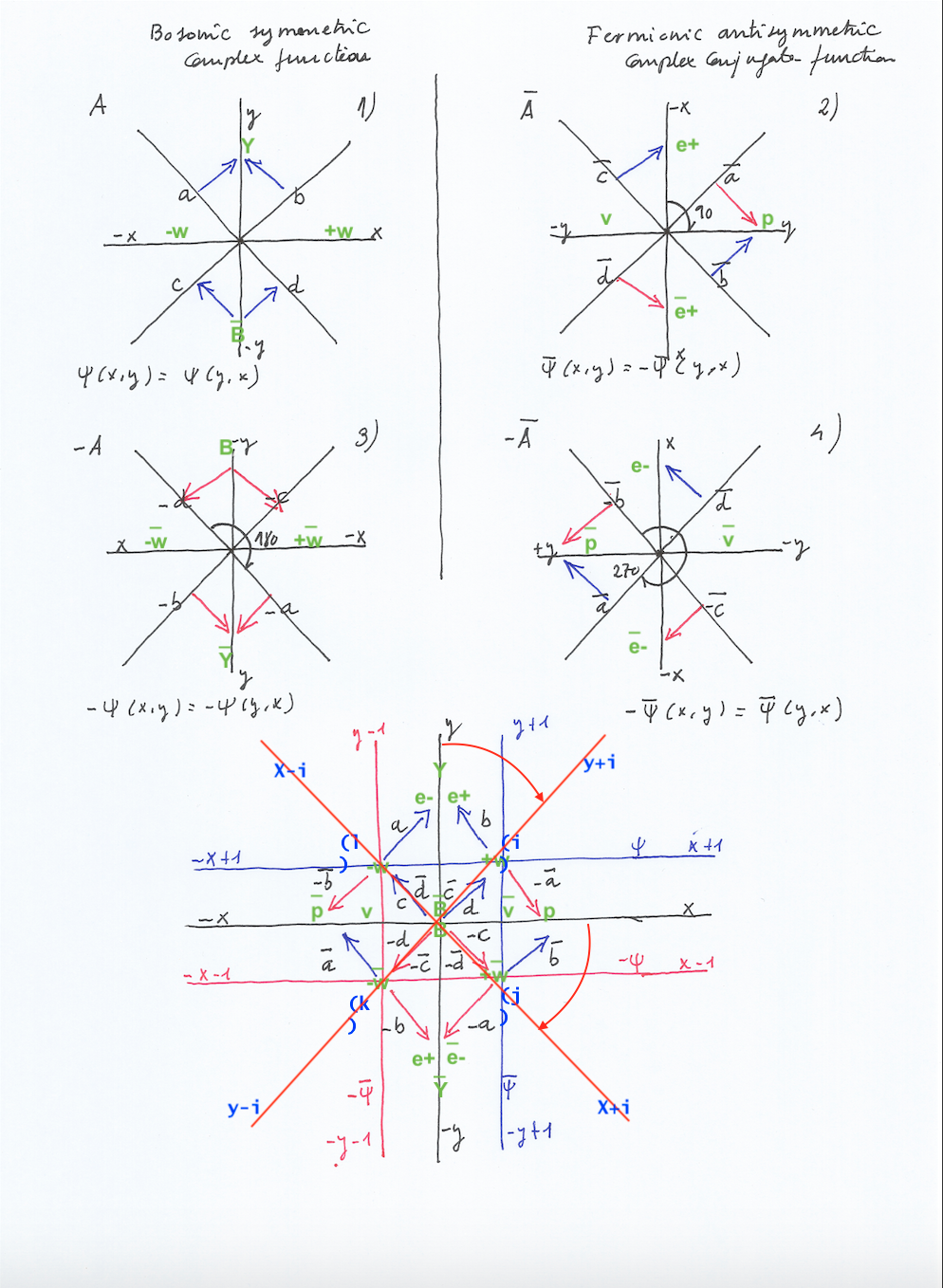
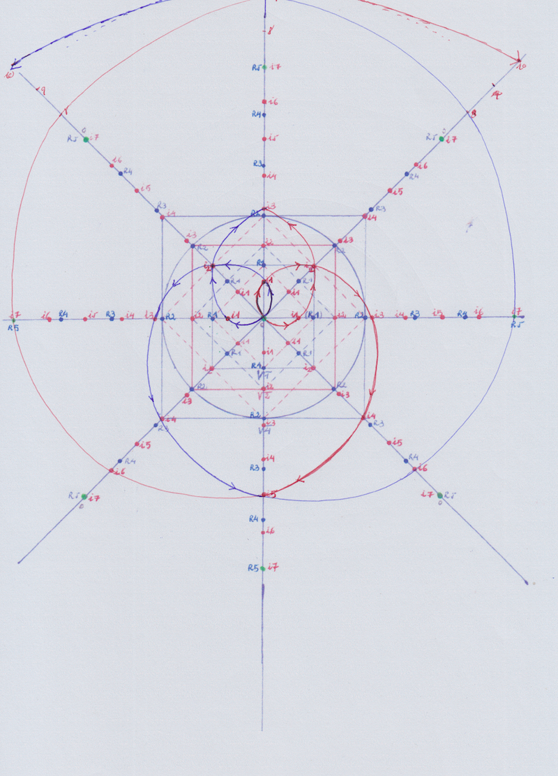
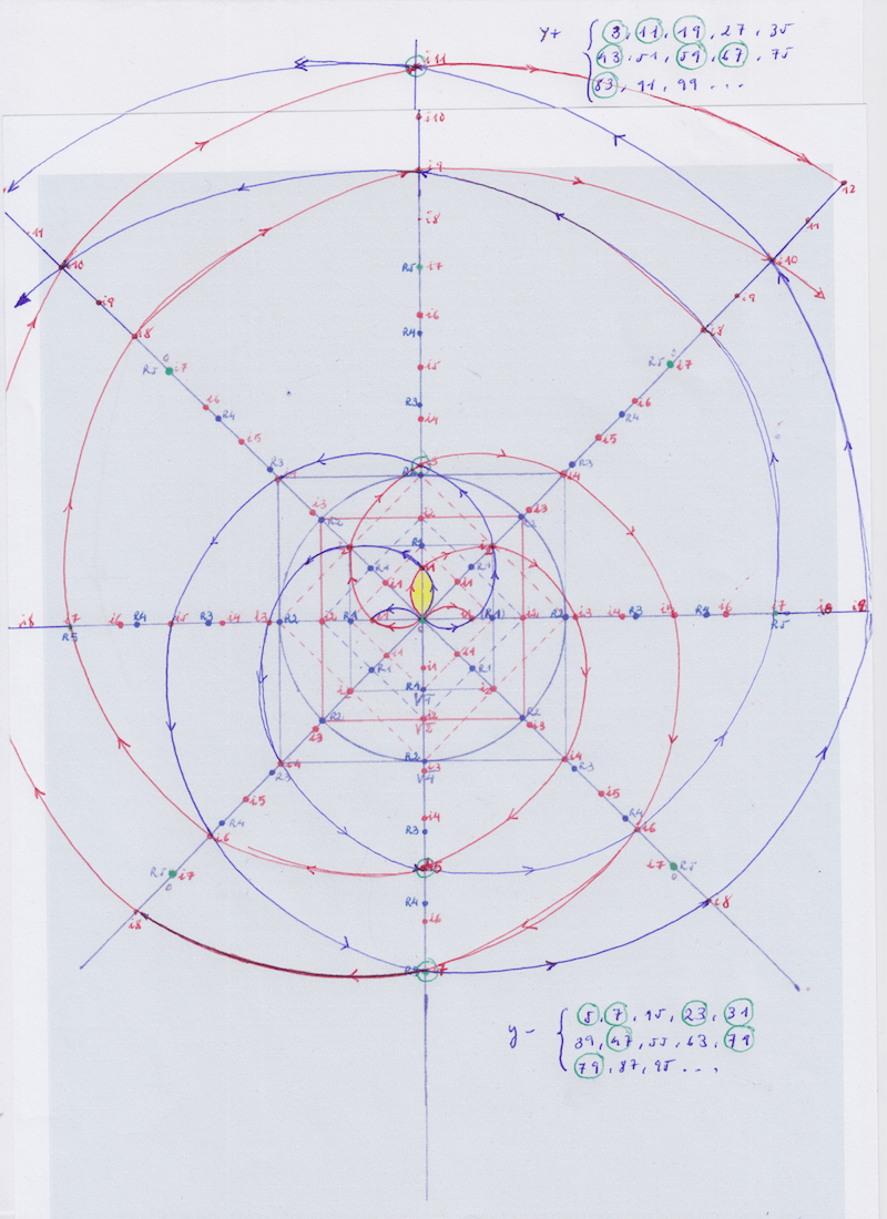
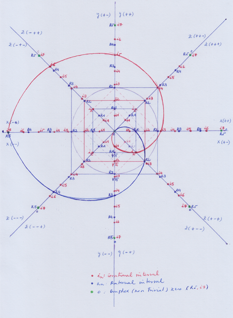
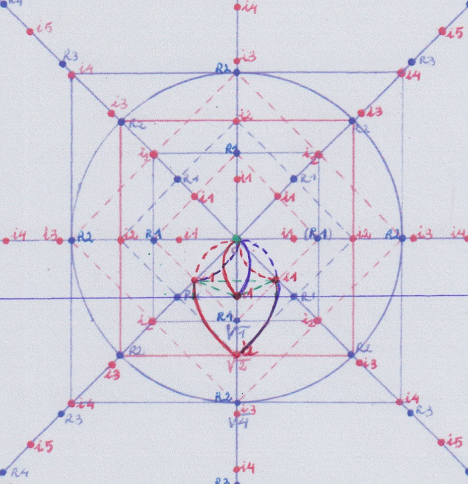
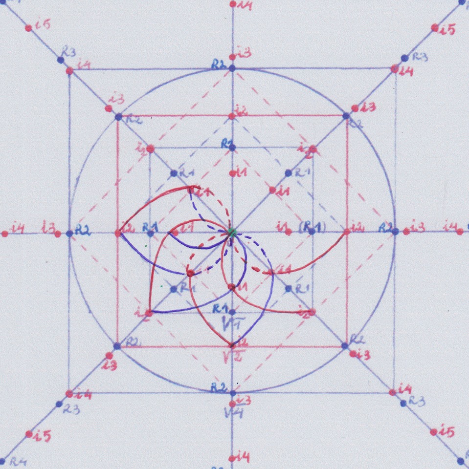
I’m going to start drawing a + curve of degree 1 and its opposite curve, a – curve of degree 1 on the Y + coordinate. The negative curve is called the «conjugate“ of the opposite sign curve. By doing this, we create a closed space, an initial field of degree 1.
Now we are going to project this initial field by prolonging its curves in a rotational way following the clockwise and counterclockwise directions, increasing the degree while rotating the coordinates, until those opposite curves converge at a point. So we can prolong them to the points Z2, +Y3, Z4, -Y5. Then, -Y5 is the point of degree 5 where those curves converge creating a field of degree 5 that is inverse with respect to the initial field of degree 1.
(When prolonging the curves I’m following the same kind of interval represented by the red dots that divide all those coordinates, as I will clarify later).
If we continue projecting the initial field of degree 1 by projecting in a rotational way its prolonged curves to the next converging point, we see the next convergence takes place at thge 9 degree on Y+. So we have a new extension of degree 9 that includes inside the extension of degree 5 and the initial field of degree 1:
We can follow creating increasing extensions indefinitely without problem. But the issue that appears now is the inverse Galois problem, how can we create – if it is possible – or how can we recognize – if they already exist – the subextensions of a lower degree between the already created extensions and the initial field of degree 1 to preserve the continuity of the symmetry when increasing the degrees of the extensions?.
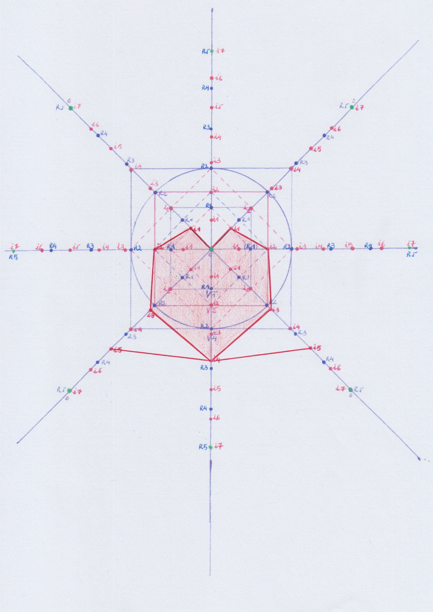
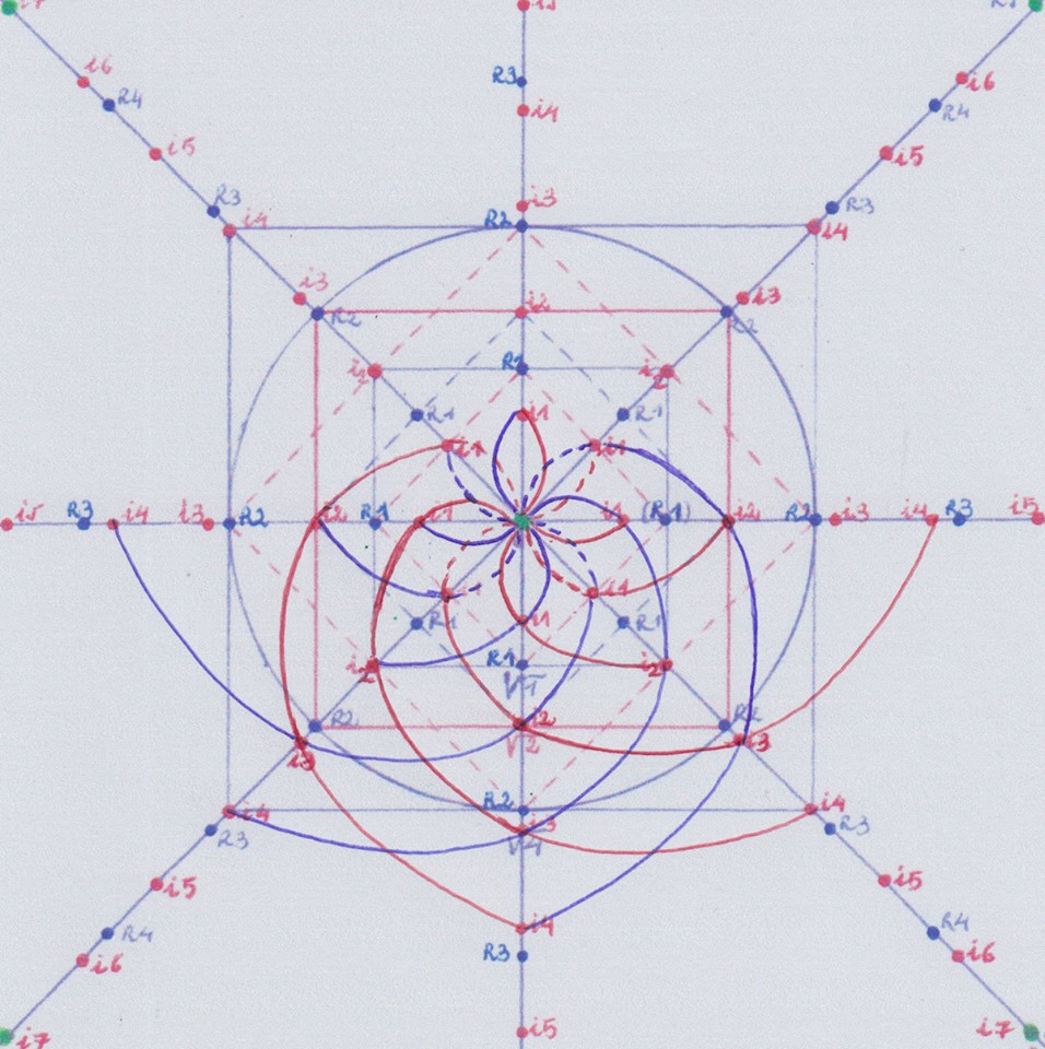
We cannot do it by projecting the initial field of degree 1 formed by the conjugate curves of degree 1 in the way we did it so far. To build the intermediate extensions or subextensions we will need to replicate the initial body of degree 1 or a half part of it, by creating new fields of degree 1 that are the image of that field. We can do that in several ways, following the reflecting symmetries, its mirror symmetry and mirror inverted symmetry, of that initial field.
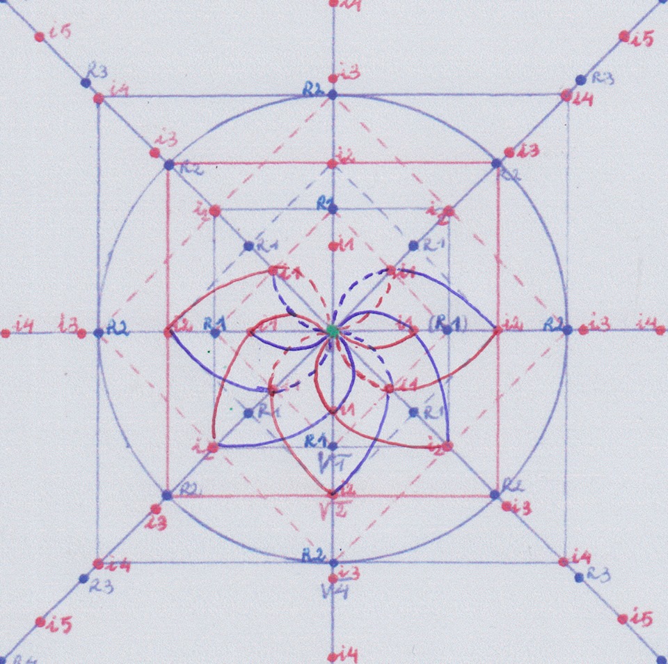
Then, we are going to draw two new fields of degree 1 on Z + and Z- that are a mirror reflection of the initial field of degree 1 that exists on Y +.
The degree 1 field on Y is a real field; its mirror reflected fields on Z are complex fields. The Z + field is the conjugate field (it has its inverse sign) of the Z – field and vice-versa.
So we have a real field of degree 1, a complex + field of degree 1, and a (complex) conjugate – field of degree 1.
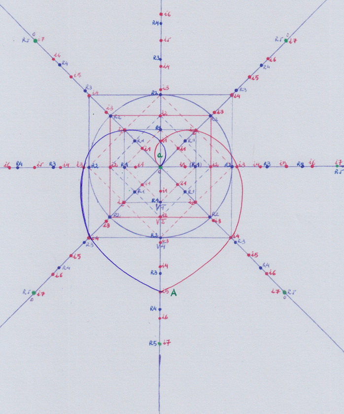
Now, by prolonging both the + and – curves of the complex and its conjugate fields, we can get new extensions that are going to form a group of symmetry that is different than the group of extensions formed by prolonging the + and – curves of the real field of degree 1.

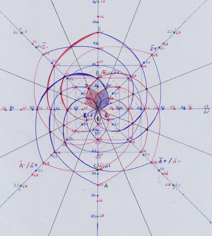
If we observe (that’s mainly what analysis is about) these figures we see how the new extensions have been formed and what different groups of symmetry already exist:
– Combining the prolongations of the + curve of the complex + field of degree 1 and the curve of the – complex field of degree 1, we form a real extension of degree 2 on Y+
– Combining the + and – curves of the complex + field of degree 1, we form a complex – (and inverted) extension of degree 5.
– Combining the + and – curves of the complex – field of degree 1, we form a complex + (and inverted) extension of degree 5 (conjugate of the – complex field of degree 5).
– Combining de + curve of the complex + field of degree 1 and the – curve of the real + field of degree 1, we form a complex + extension of a degree that is intermediate between 1 and 2.
– Combining de – curve of the complex – field of degree 1 and the + curve of the real + field of degree 1, we form a complex – extension of a degree that is intermediate between 1 and 2, (conjugate of the + complex field of this same intermediate degree).
By creating those extensions of an intermediate degree we added two new coordinates between the existing Y and Z coordinates.
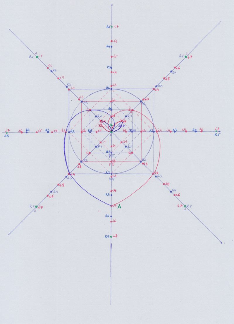
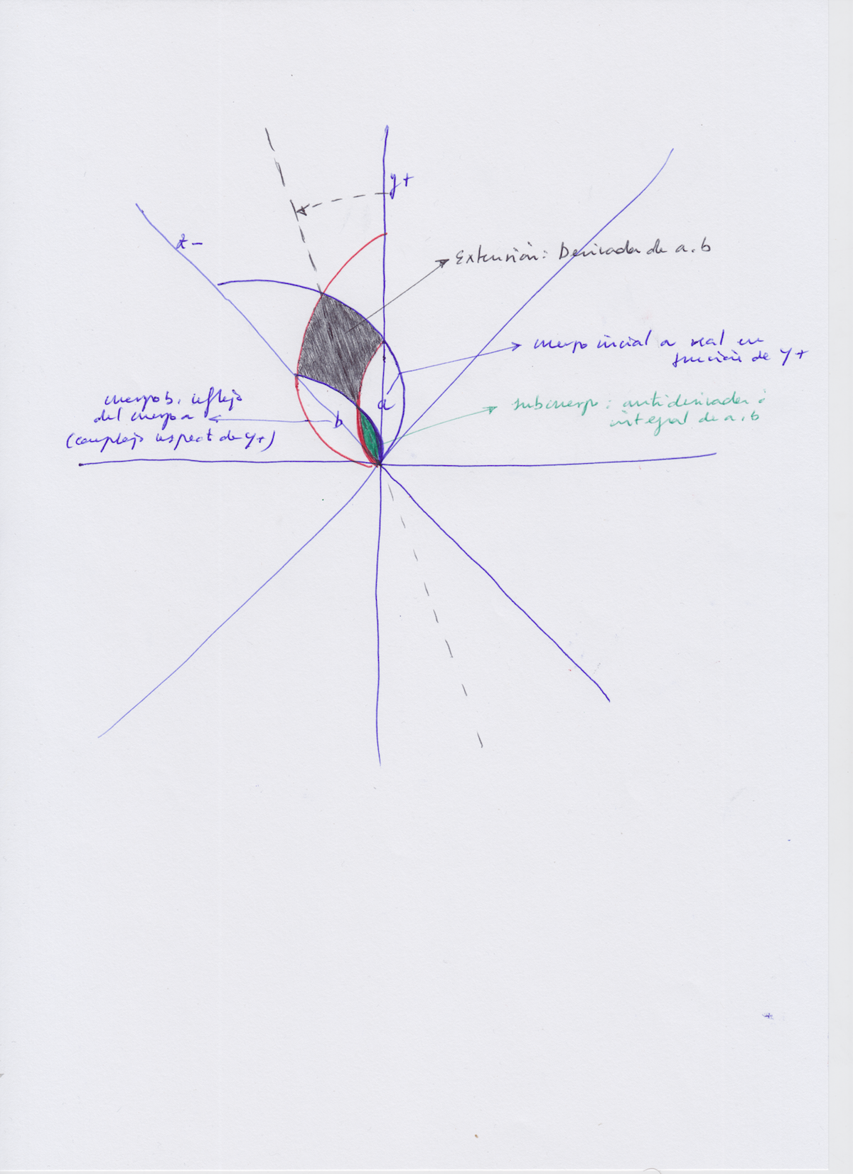
This two last extensions we formed by combing a real and a complex part are very interesting because there, the real field Y1 acts as a complex body which is conjugate of the another complex body of degree 1 on Z; they both determine the structure of the new intermediate extension whose center of symmetry is a new coordinate we create by displacing, rotating Y+ towards Z, so they are not trivial fields with respect to that intermediate extension.
By doing that, we have created at the same time a subfield of a degree lower than 1 between the real field of degree 1 and the complex field of degree 1. That subfield will be real with respect to the center of symmetry that is the coordinate displaced from Y towards Z, and trivial with respect to the created extensions (It does not determine the structure of the created extension), but at the same time, when being considered from the perspective of the real Y coordinate, it will be a complex subfield that is not trivial because it determines the structure of the half of the real field of degree 1 and half of the complex field of degree 1.
Then that subfield is a very interesting structure because it is inverse with respect to the created extension: First, from an initial field of degree 1 on Y we created their complex reflected fields of degree 1 on Z; Then, from the real field of degree 1 and its complex field of degree 1 we create a new extension on a coordinate that is displaced from Y towards Z; and at the same time we get a subfield respect to which the real and complex fields of degree 1 are their extensions. Following the path of the increasing extensions we would get infinitely big extensions while following the path of the decreasing subfields we would get infinitely small subfields.
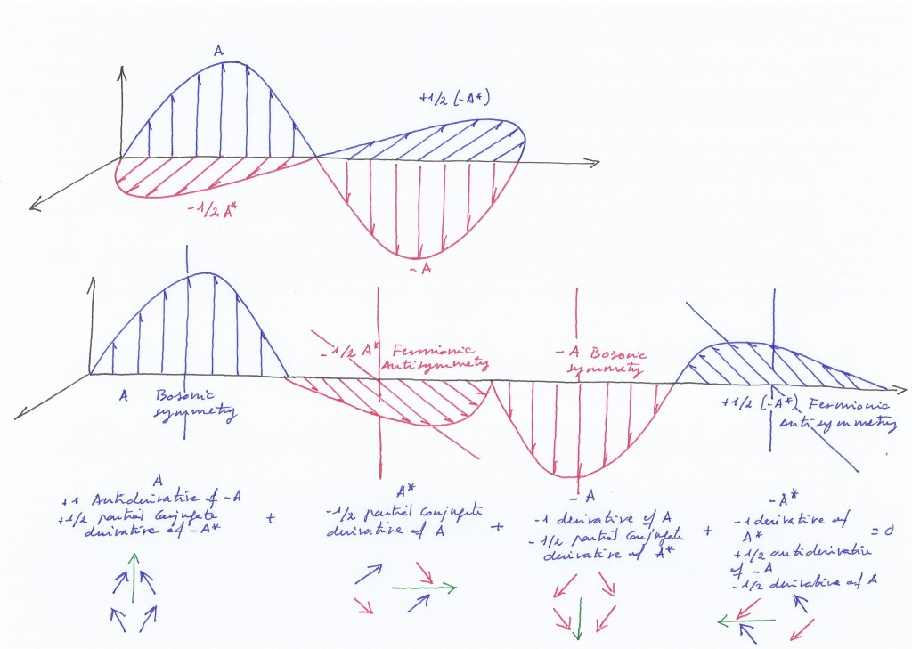
In this sense, if we called «derivative» of the real and complex fields of degree 1 to the increasing extension we created on the displaced coordinate by projecting those fields in a rotational way, the decreasing subfield we also created at the same time by doing that would be the anti-derivative of that real and complex fields of degree 1.
So we could already use the terms that are used when it comes to differential equations: The anti-derivative we get by combining the projections of the real and complex fields of degree 1 would be their integral».
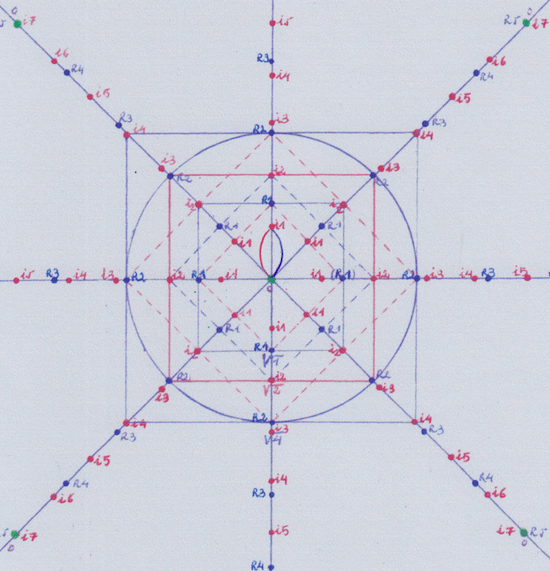
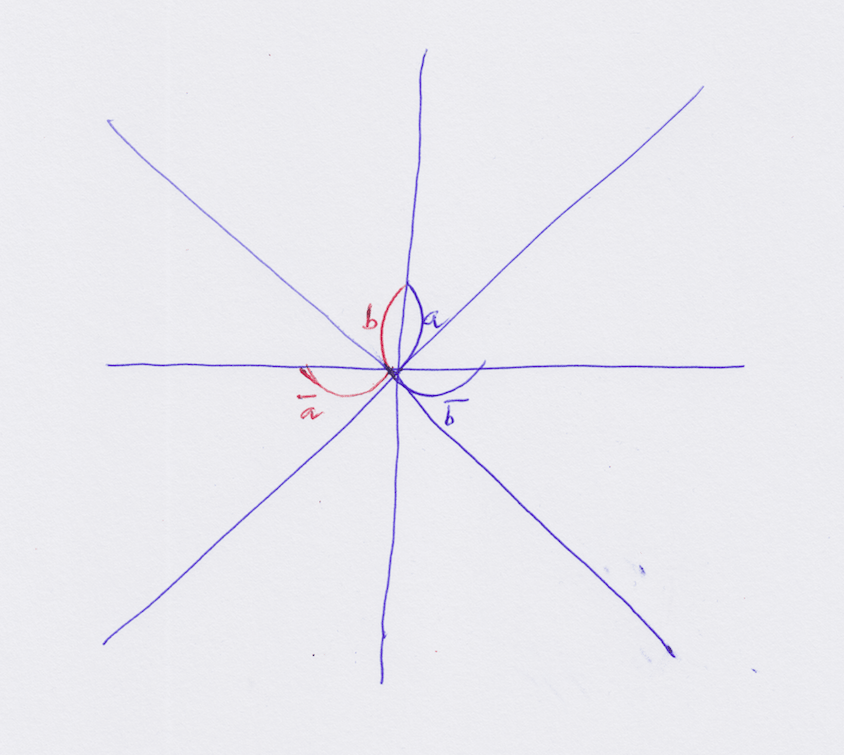
To see this clearer I drew another figure (on the above diagrams it’s not clearly visible) where I colored in green the antiderivative subfield of «a» and «b», and I drew in black the derivative that would form – with the included real and complex fields of degree 1) the projected extension.
The real and complex fields are the antiderivative of the extension, but the antiderivative of the real and complex fields is its shared subfield.
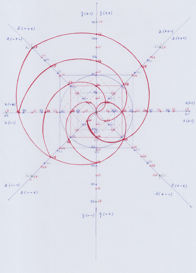
[I think the function (or functions) represented on the above figure could be related to the Riemann Z function: the coordinate where the z function’s non trivial zeros would be placed would be the displaced coordinate that is the center of symmetry of the derivative and the antiderivative of the real and complex fields a and b. The converging points of the curves would be the zeros of the Riemann function. The Riemann non trivial zeros are those that have a real and a complex part, and in this sense we can think as non trivial zeros the points where the curves converge to create the derivative and the antiderivative, because the converging curves are a prolongation of the real and complex fields.
But I think it’s not a coincidence that when it comes to Galois groups and extensions of a field mathematicians are speaking about the trivial and non trivial structures depending on if they determine the structure of the extension.
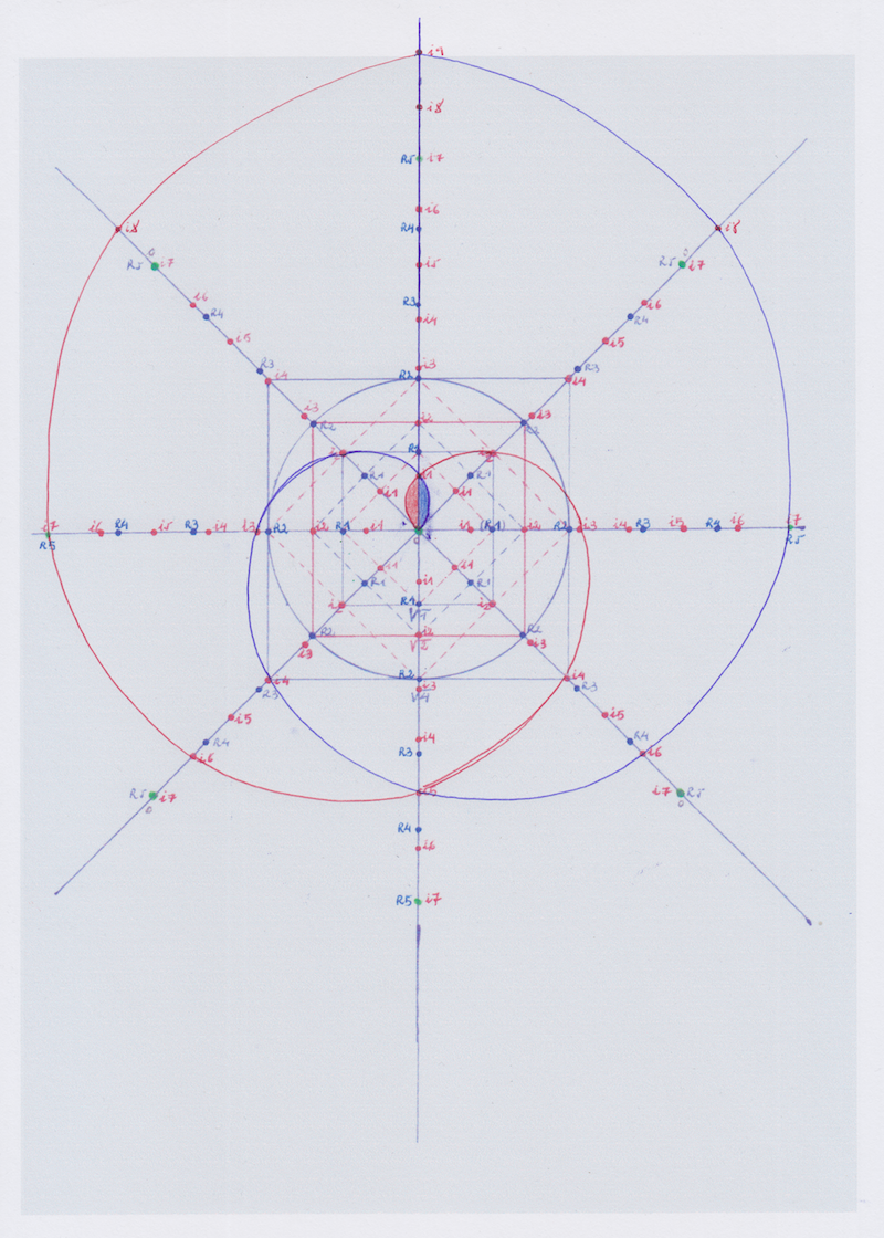
In this sense, it’s also interesting that the integral subfield is at the same time real and complex, depending on the center of symmetry we set our focus, the real Y coordinate, or the displaced coordinate. The zero point that represents the convergence of the curves of the integral passes through a region that is not the real coordinate Y nor the complex coordinate Z, but an intermediate region that is the 1/2 the complex plane.
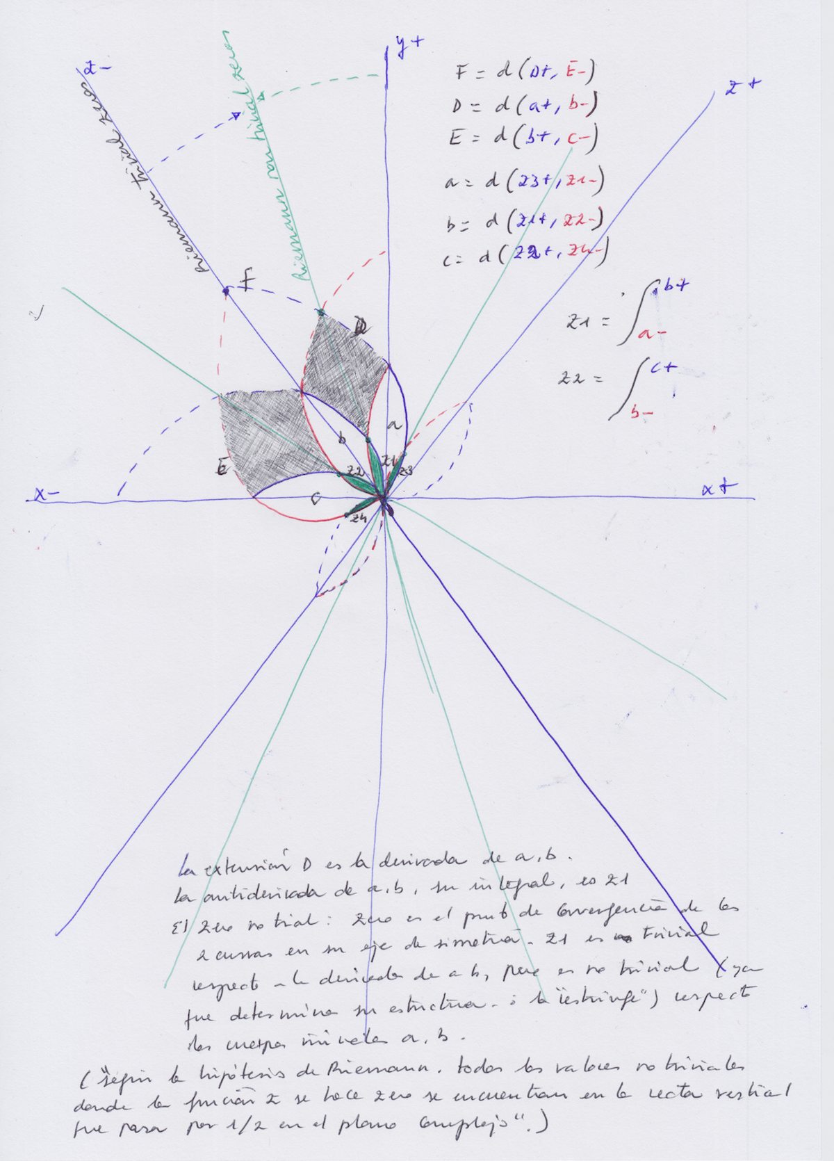
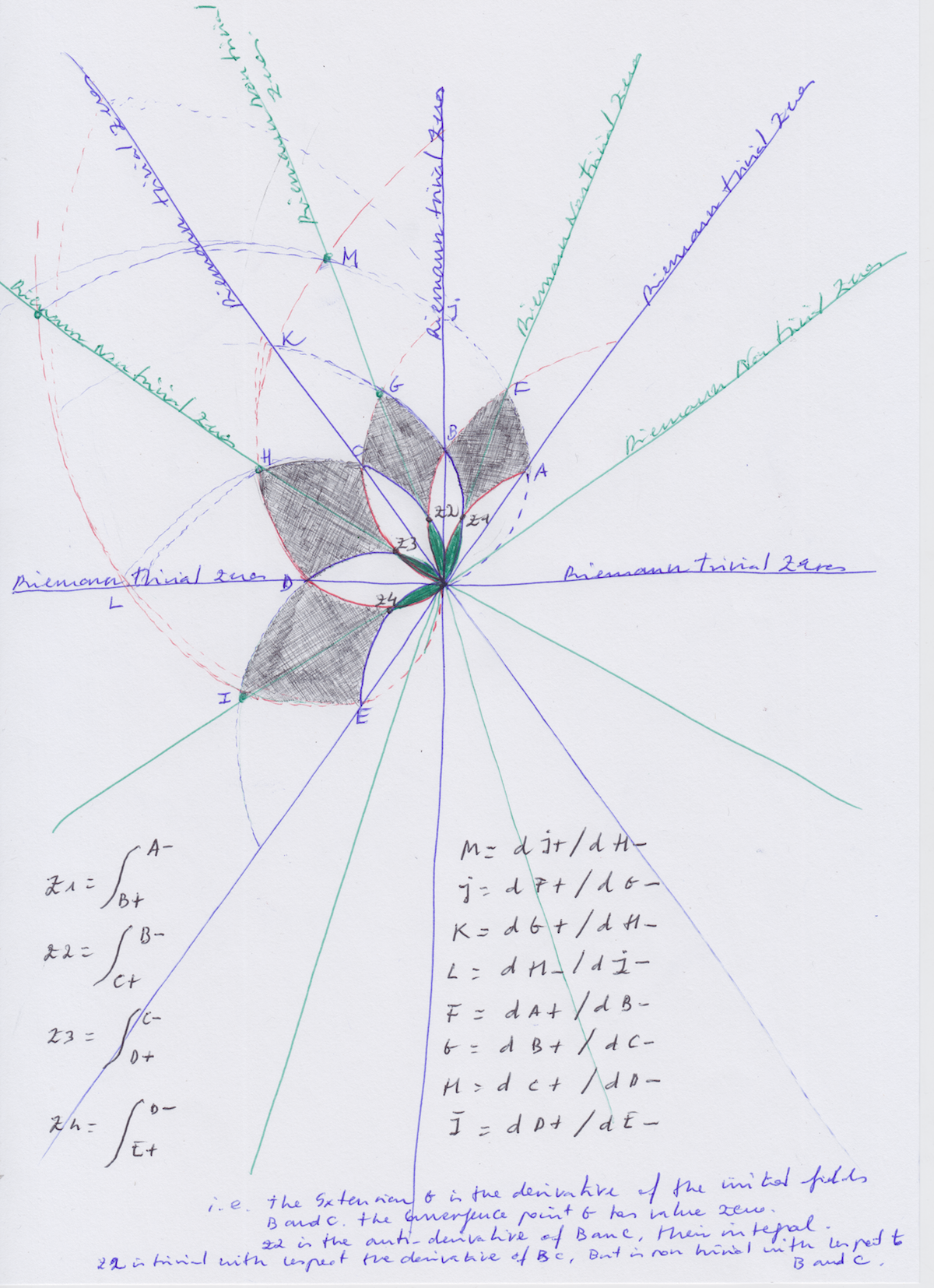
The Riemann hypothesis states that all the non trivial values where the Z function becomes Zero, are on the straight line passing through 1/2 the complex plane. I set on green color that line passing through 1/2 the complex plane where some curves converge getting a zero value. The green field z1 on that line is non trivial with respect to the extensions whose structure it restricts or determines.
It may seem too speculative to consider these diagrams can represent the Riemann Z function, but anyway I think they are not very far from it. Reading the Riemann work “On the hypotheses which Lie at the Bases of Geometry», it’s possible to follow easily some paragraphs by visualizing the diagrams I attached above and will attach below. Actually, it seems as if Riemann were visualizing in some way these kinds of intersecting structures.
You can take a look at the famous Riemann text here: http://www.cs.jhu.edu/~misha/ReadingSeminar/Papers/Riemann54.pdf
or https://www.maths.tcd.ie/pub/HistMath/People/Riemann/Geom/WKCGeom.html
And you can visualize an example of Riemann manifold and submanifold in this figure attached in the Wikipedia about the «Riemann manifolds» («Variedades de Riemann» in the Spanish version):
https://es.wikipedia.org/wiki/Variedad_de_Riemann

To me, the terms «manifold» and «Submanifold» have the same meaning than «extension» and sub extension».
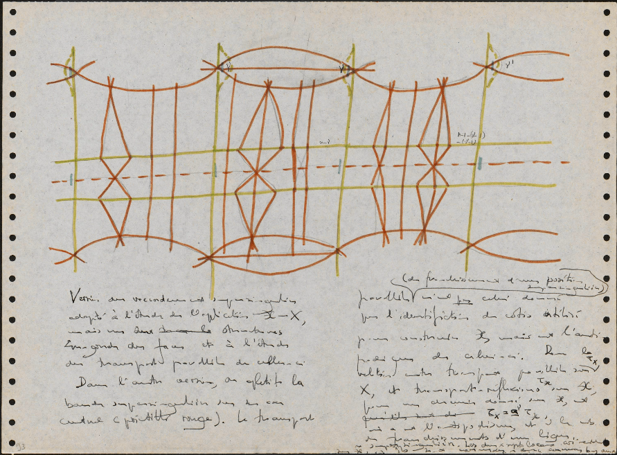
If you still do not see clearly that the figures I’m attaching in this post are related to the Riemann’s geometry you can take a look at the drawings that Riemann himself did speaking about connected surfaces in his work about Abelian functions:
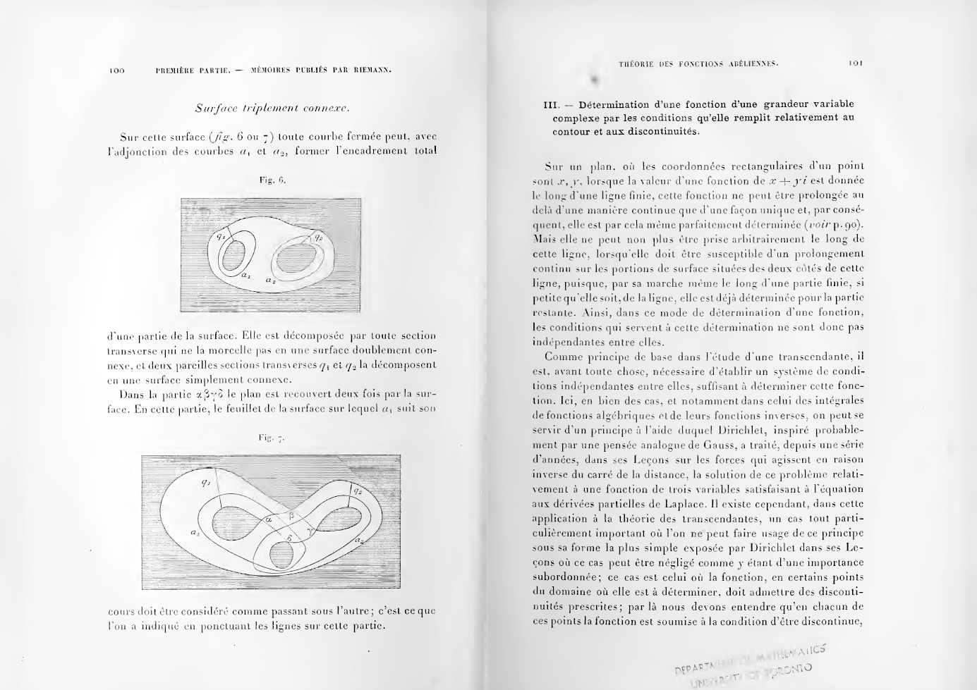
I took it from his mathematical works at https://archive.org/details/oeuvresmathmat00riem
And you can compare it with this another figure I made:
It’s almost the same thing.
What is interesting to me looking at the Riemann’s drawings is that it’s clear Riemann did not arrive to his notion of space and connected surfaces starting from the analysis of geometric figures – he could have started by simply drawing and analyzing spirals of opposite sign that start from different spatial coordinates as I did – but he started instead from some kind of imaginative envision he had from which he was able to concrete his rudimentary drawings for expressing his ideas about connecting surfaces. He did not have much time to concrete his multiple and imaginative intuitions.
As Riemann’s ideas were considered subsumed in later and more accurate works, it seems currently no one has a clear idea about what the hell a Riemann’s manifold is. None of the mathematicians I many times sent these figures mentioned they were Riemannian geometric figures when it’s super evident looking at this above picture that they actually are.
It’s pretty hilarious and sad at the same time.
Many of the ulterior developments related to groups, manifolds, varieties, etc seem to be almost the same thing with different names.
For example, take a look at these drawings of Alexandre Grothendieck, one of the most famous mathematicians of the XX century:
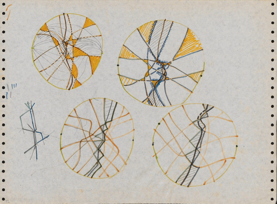
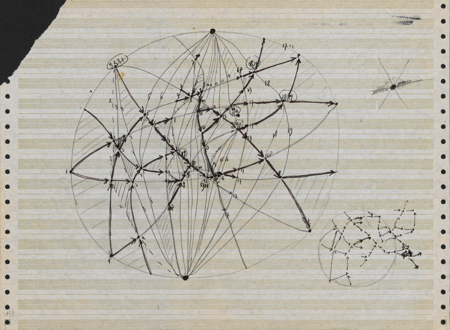
(I took those pictures from https://grothendieck.umontpellier.fr/archives-grothendieck/
[Système de pseudo-droites] : notes manuscrites (1983-1984, s.d.). Cote n° 154 (175 p.))
What do you think Grothendieck was trying to represent with them? It’s quite absurd he had to invent the expression «dessin d’enfant» (kids’ drawings) to name these kinds of drawings. You can read in wikipedia that «In mathematics, a dessin d’enfant is a type of graph embedding used to study Riemann surfaces and to provide combinatorial invariants for the action of the absolute Galois group of the rational numbers». https://en.wikipedia.org/wiki/Dessin_d%27enfant
The problem with the dessins d’enfant is that they do not let mathematicians know when their orbits belong to a Galois group and when they are not related to it. They do not show the invariants (that, in my opinion, should be given by the kind of rational or irrational metric magnitudes we divide the space with).
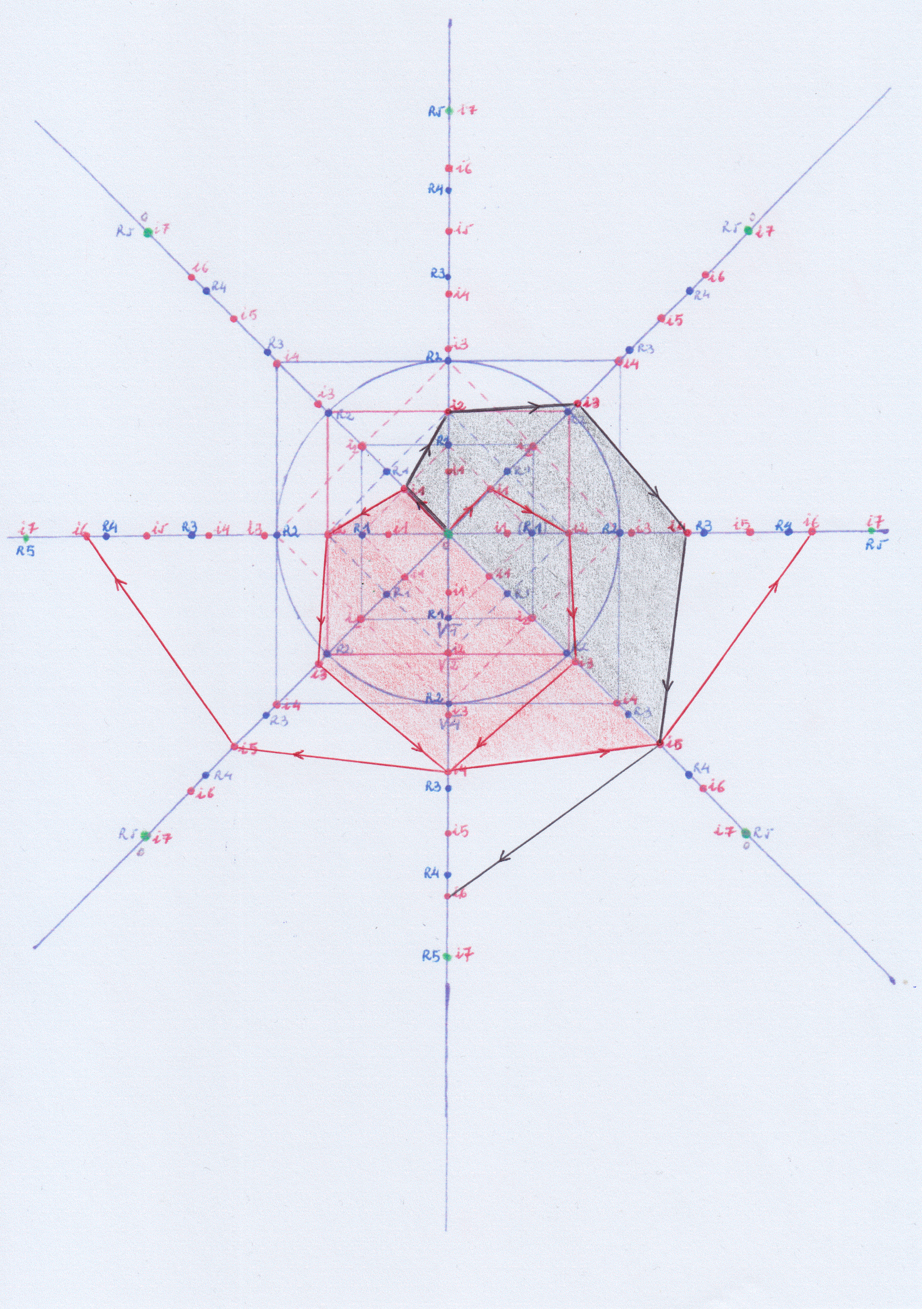
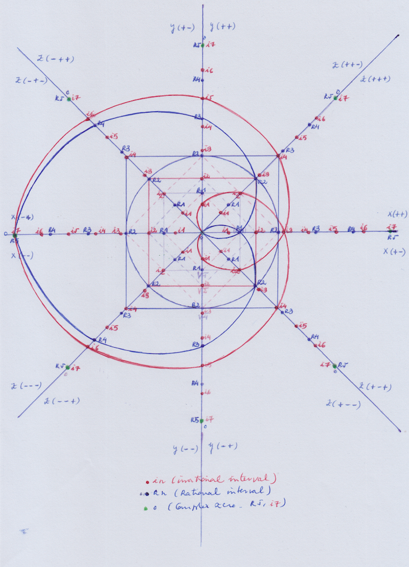
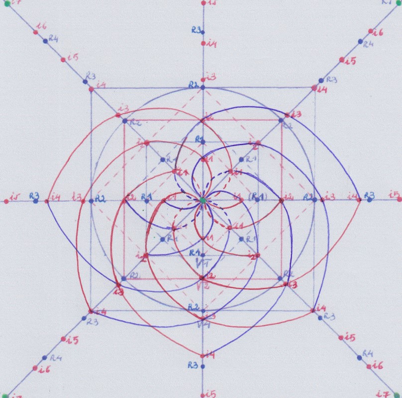
But let’s continue with the exposition by creating new extensions. We can see all the combinations that will create the different groups of symmetry, that I think would be «Galois» groups, that will be followed by the different extensions, and the Hodge cycles or shapes (that we know are combinations of algebraic curves), that will be the extensions and groups of extensions formed while creating the whole structure that has a same and continues symmetry, covering smoothly the space.
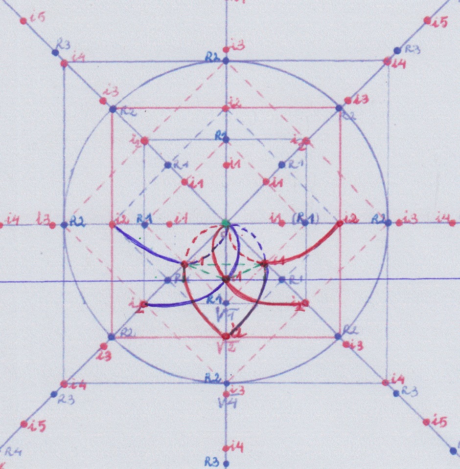
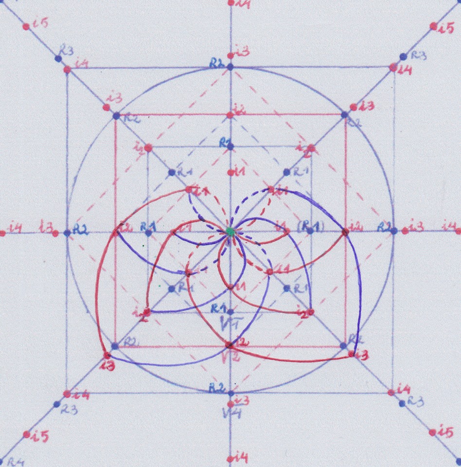
Now I’m going to replicate the created fields of degree 1 by creating their mirror-inverted fields of degree 1. By prolonging them, we will get the extensions that are mirror-inverted reflection of the previous ones:
We can continue completing this figure:
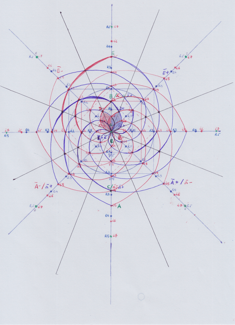
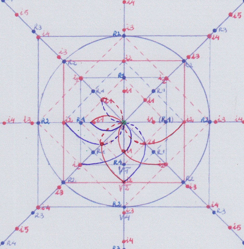
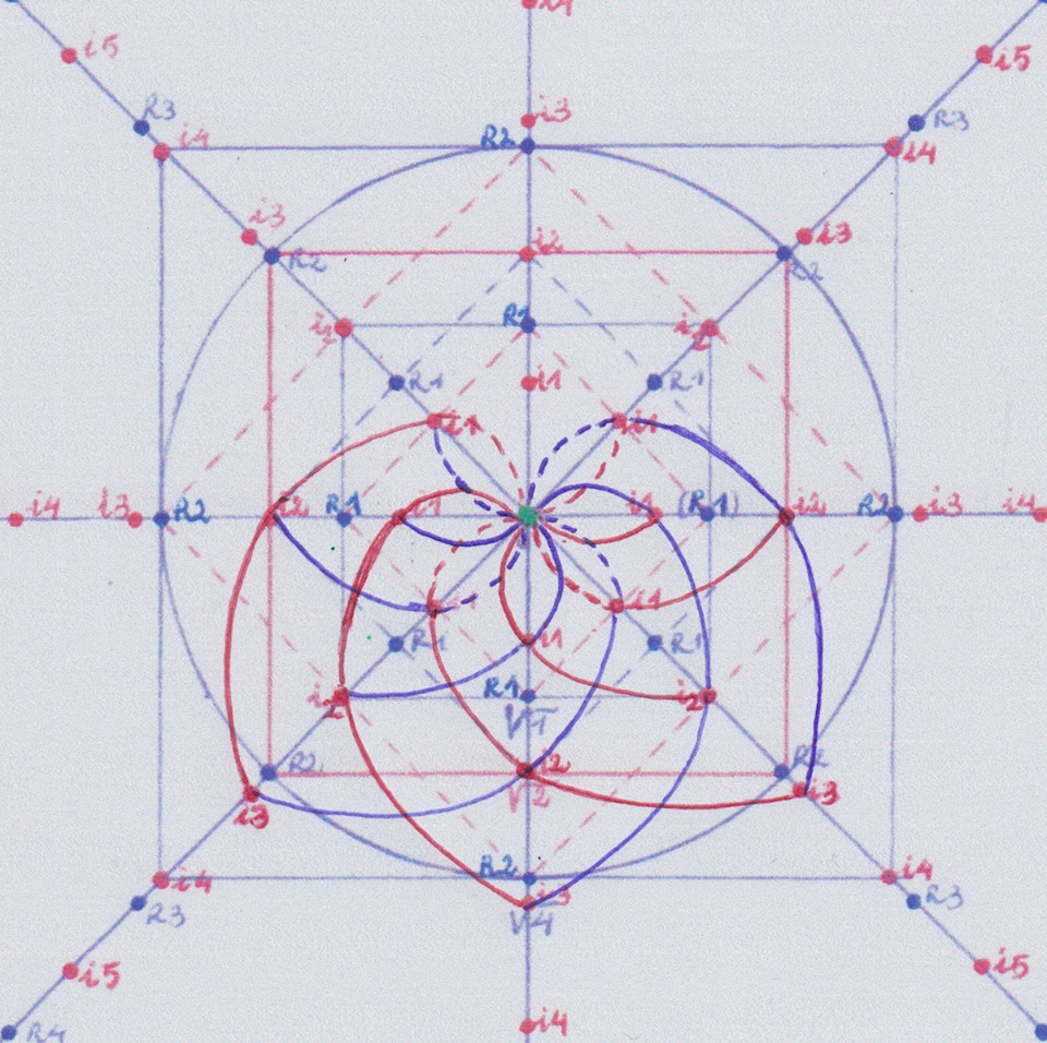
Another option that we have to form the extensions is to create the inverse curves on X of the real curves of degree 1 on Y and combine their projections when prolonging them in a rotational way.
If we form only the extensions that appear when prolonging the two conjugate curves formed on X (inverse of the real curves of degree 1), we see we will get a new group of extensions. The first extensions of that group is an extension of degree 3 on Y+, and then an inverted extension of degree 7 on Y –
It’s interesting to see that on the coordinate Y – appear in a consecutive way to prime extensions, 5 and 7, which are twin primes. They both follow groups of symmetry different. So we are going to research a bit more about this.
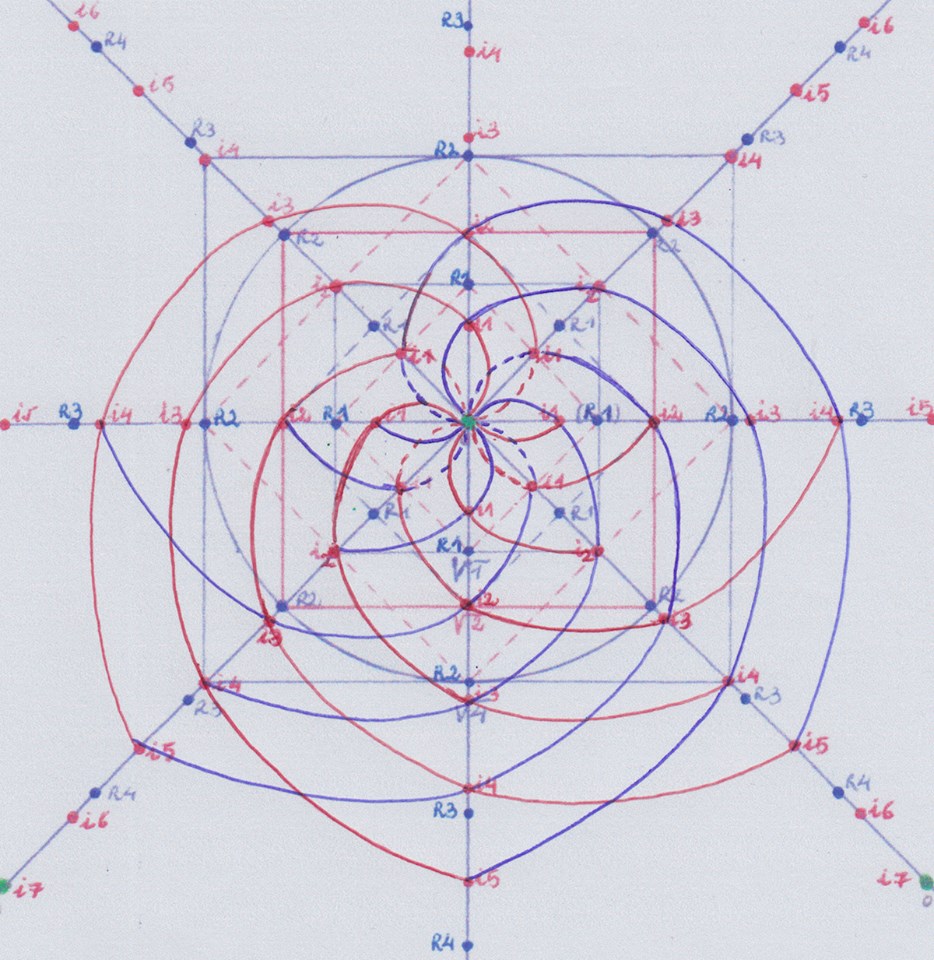
If the group of symmetry of the extensions formed by prolonging the conjugate curves of the real field of degree 1 on Y (which forms the extensions of degree 5, 9, 13, 17, interferes with the order of the prime extensions that follow the group of symmetries of the inverse curves on X = and X -, if we select only these last extensions we should avoid interferences on the primes distribution.
So now we are going to get only the extensions formed in a polar way on Y + and Y – following the – and + curves of degree 1 we created on X:
If we confront the resultant extensions on two rows we see they are 6 primes on each row, and that there is a relation of mirror inverted symmetry between the elements that form opposite couples:
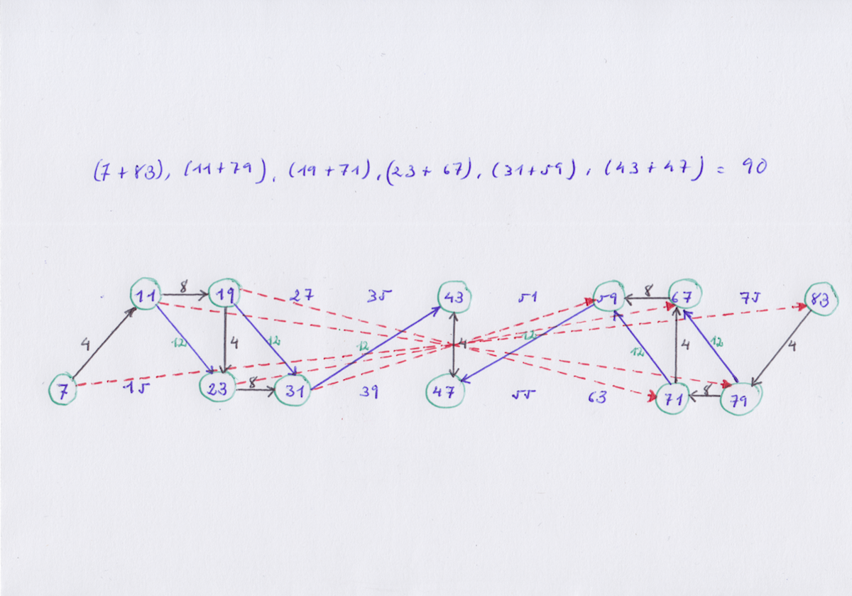
Each element added to its inverse couple is = 90.
I found this same kind of correspondence as an example of the correspondence between Galois extensions in this book about Abstract Algebra (by Charles C Pinter):
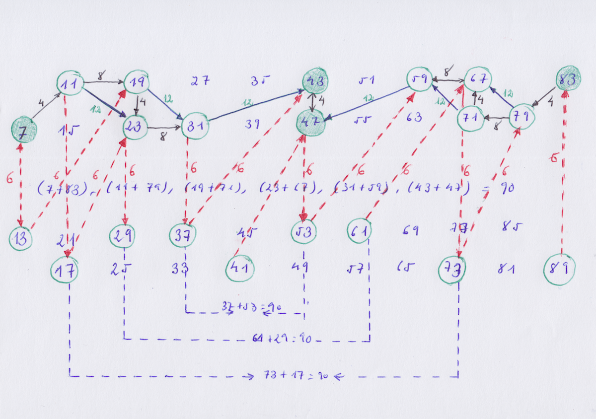
If we also add two other rows with the prime extensions that appear when projecting or prolonging the + and – curves of the real field of degree 1,
we see that the distribution also follows a short of order:
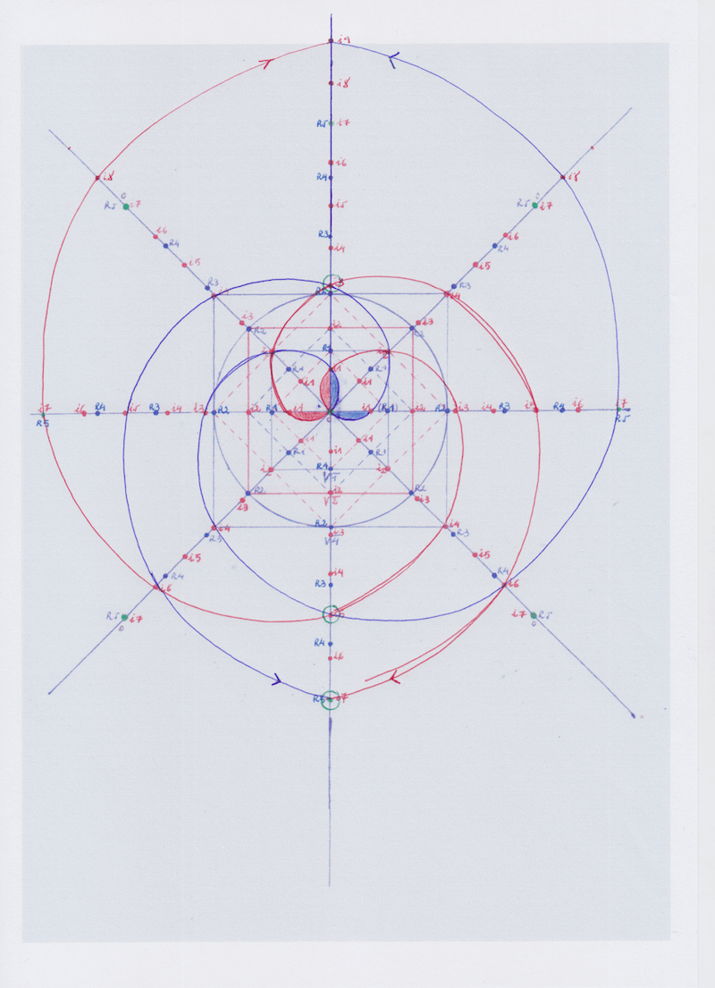
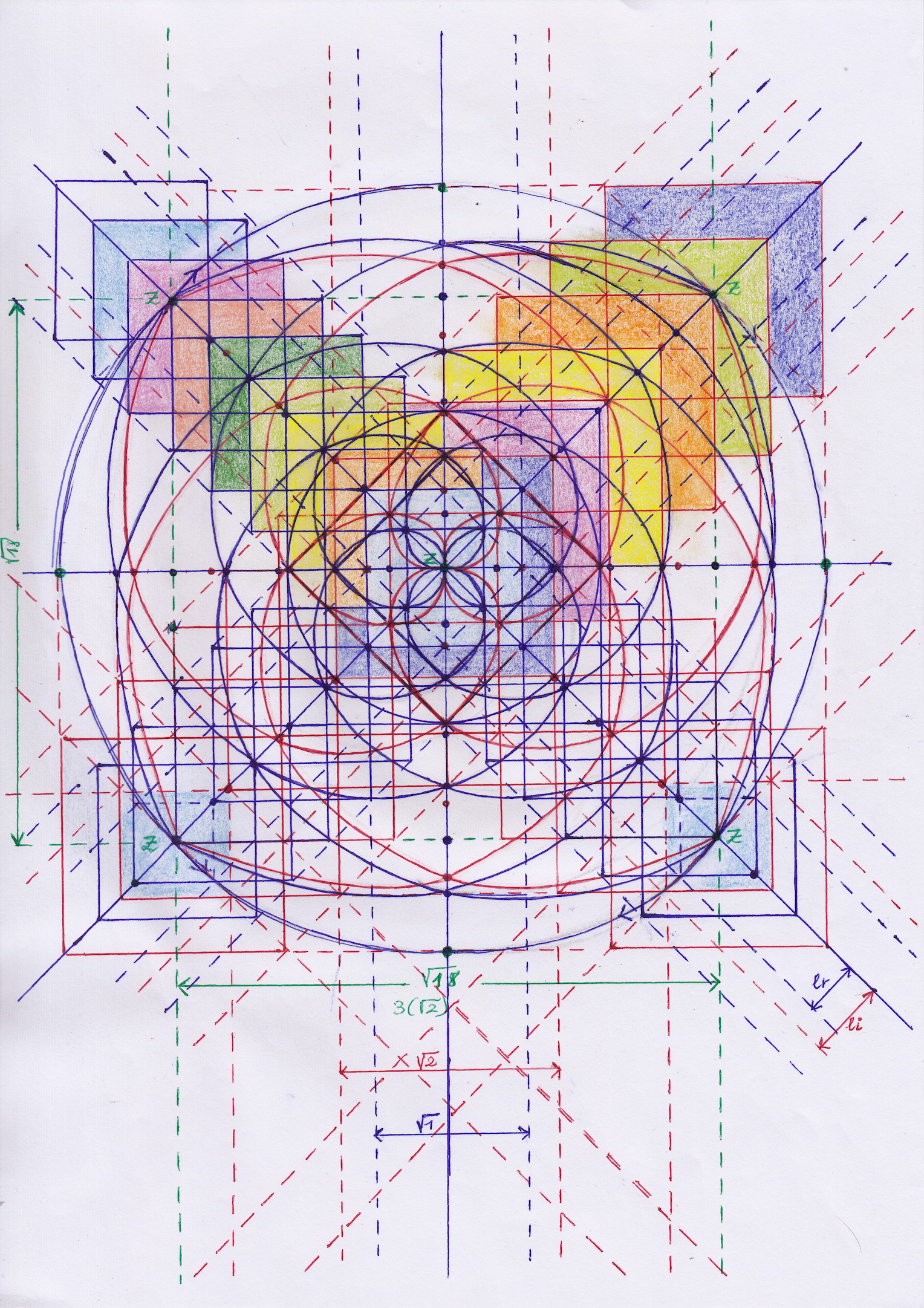
On the other hand, I represented the diagrams with curves, but they also can be represented in a similar way by using straight lines in this way:
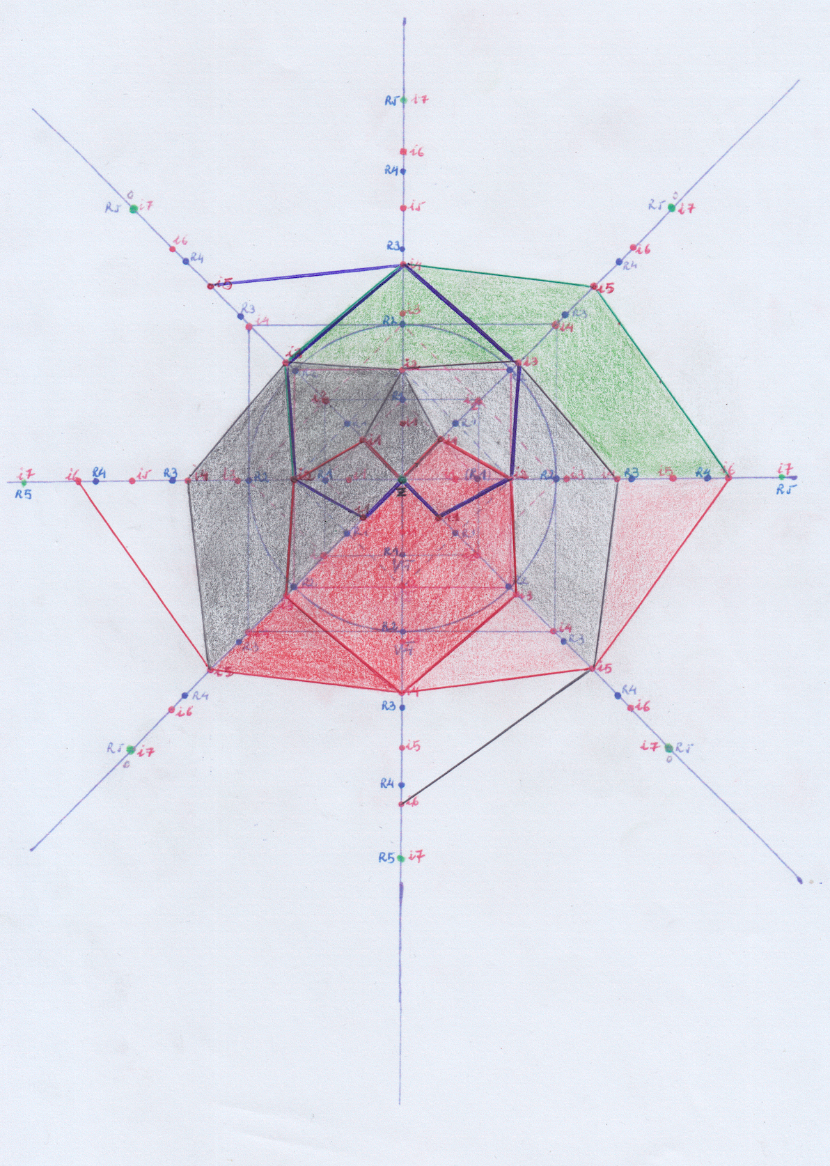
Another way to represent the extensions is this one:
In all these figures I followed the interval that we get when measuring through Z a segment from the center of circumference to the center of the square of area 0.25; Repeating that interval through Z we arrive to the center of the square 1 and to the center of the square 4. I think that would be an irrational interval.
But it’s also possible to get another kind of interval when measuring a segment from, the center of the circumference to the center of the square 0.50. It’s the same interval followed by the square of area 2 and I think it would be rational.
Combining those intervals when creating extensions we also get mixed extensions. But the intervals cannot be combined in an arbitrary way if we want to keep the symmetry. Those intervals are not directly comparable or interchangeable, although they both converge periodically at the 7 irrational and 5 rational degrees.
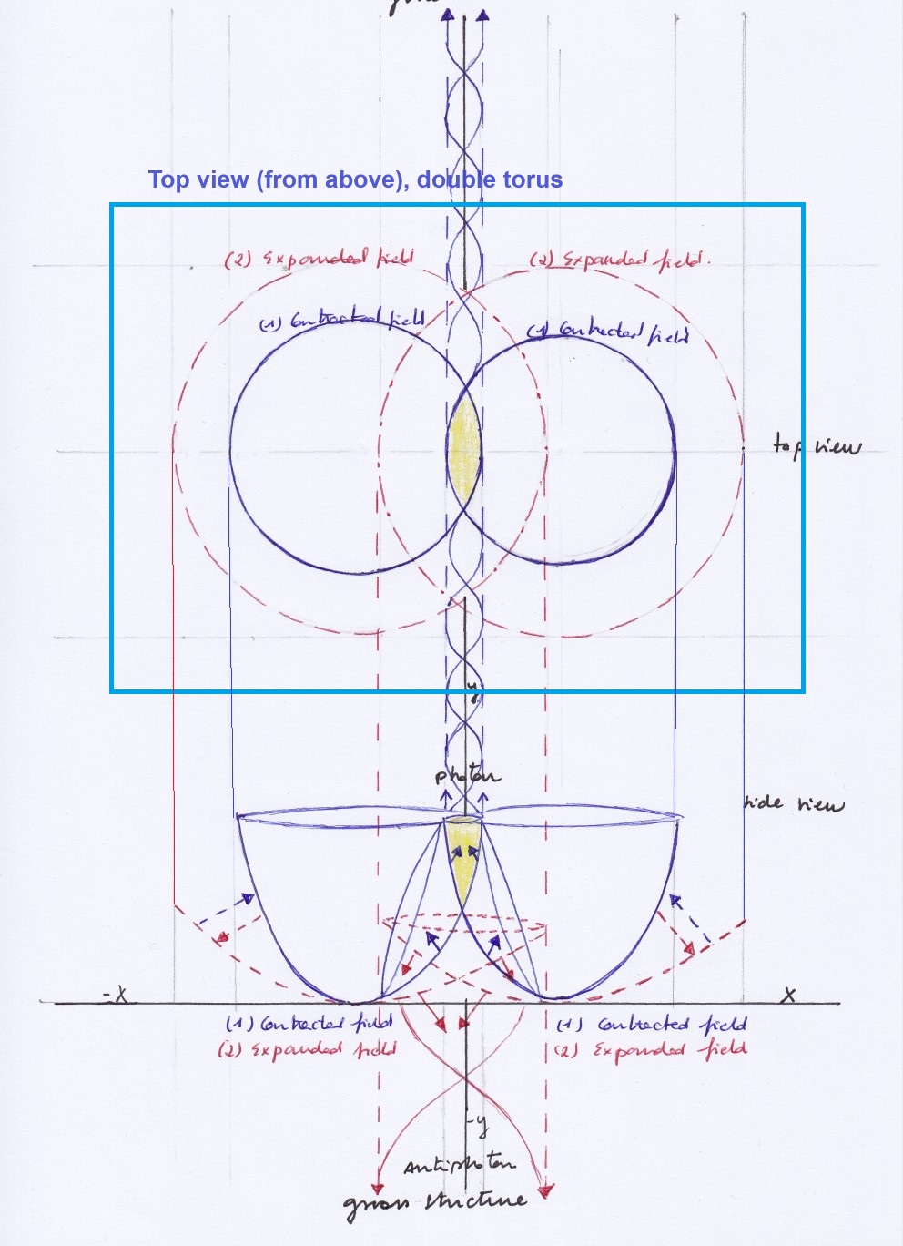
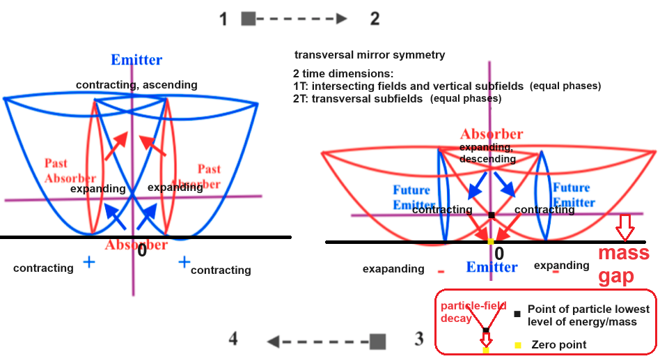
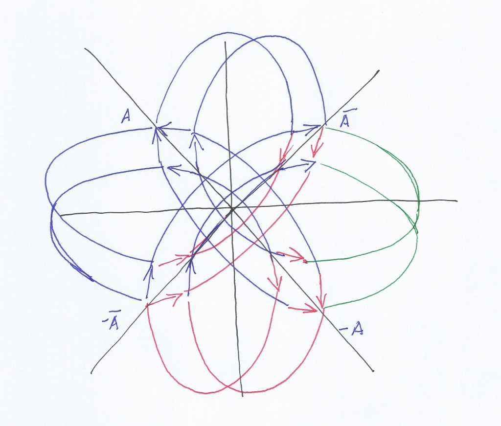
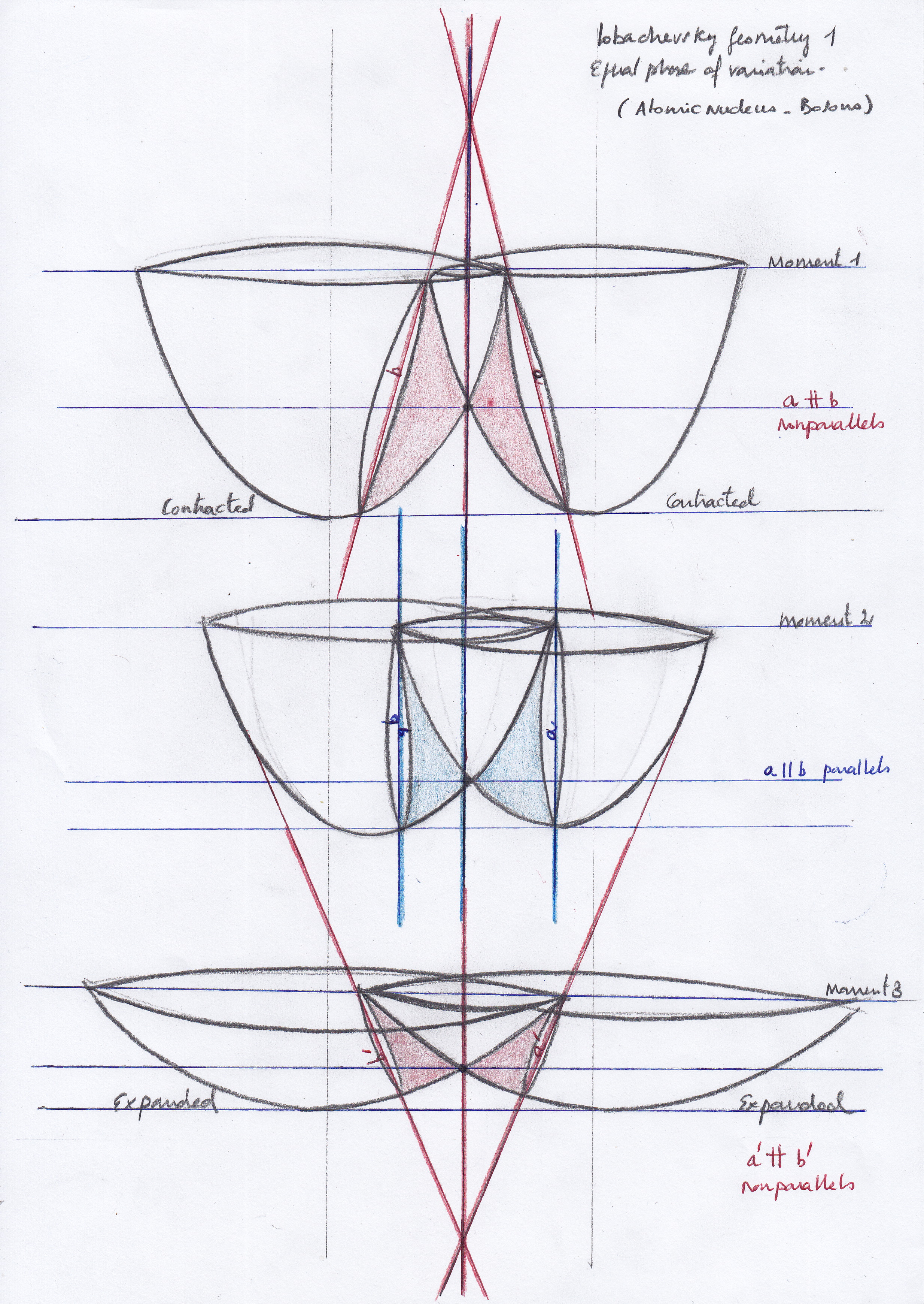
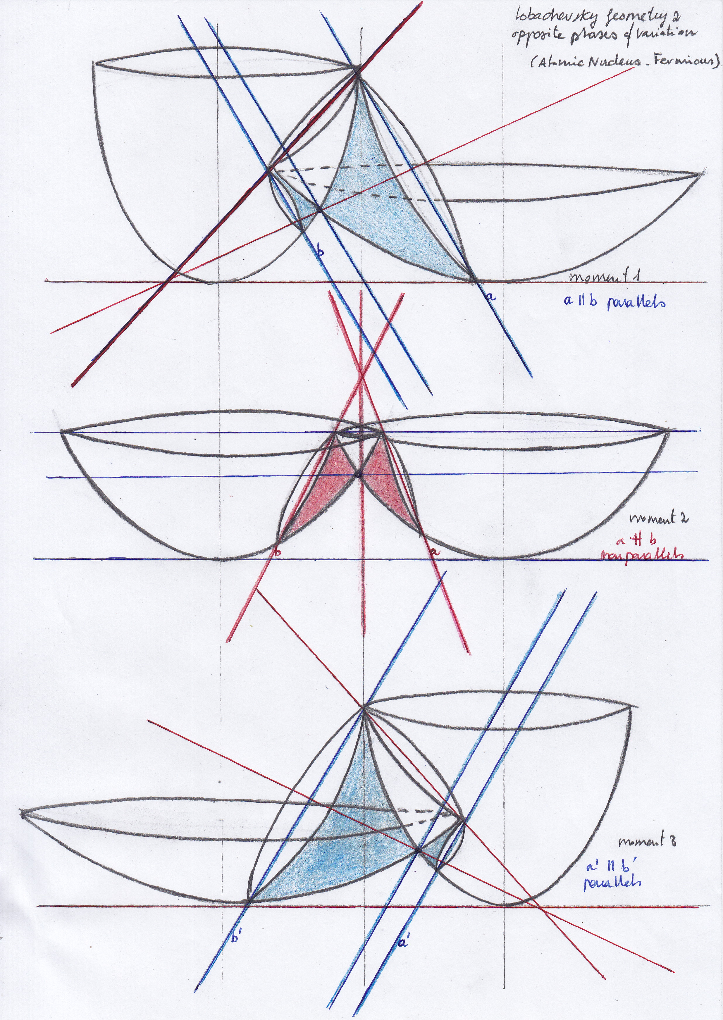
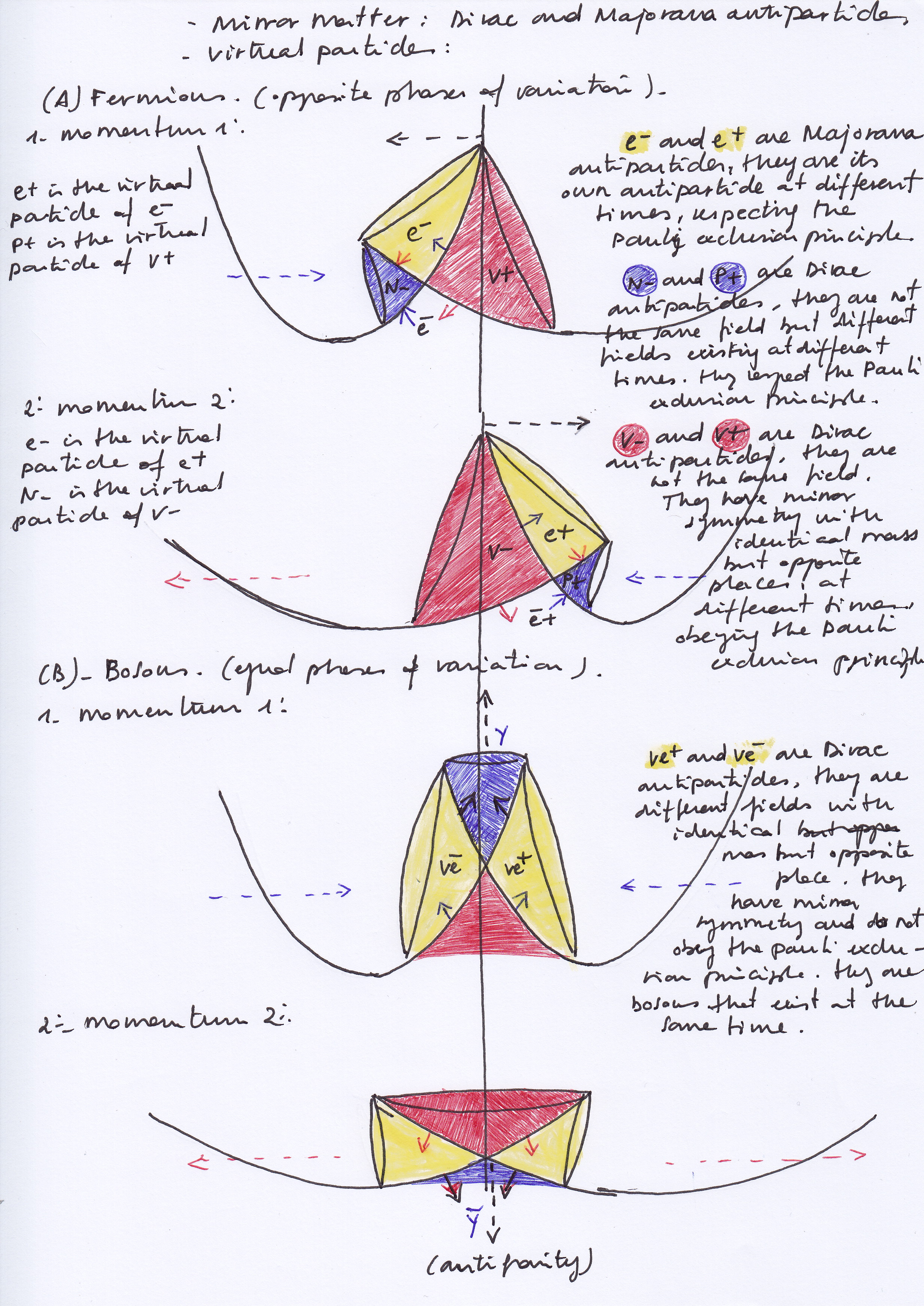
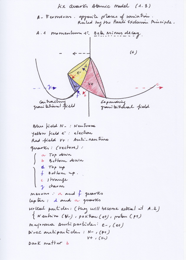
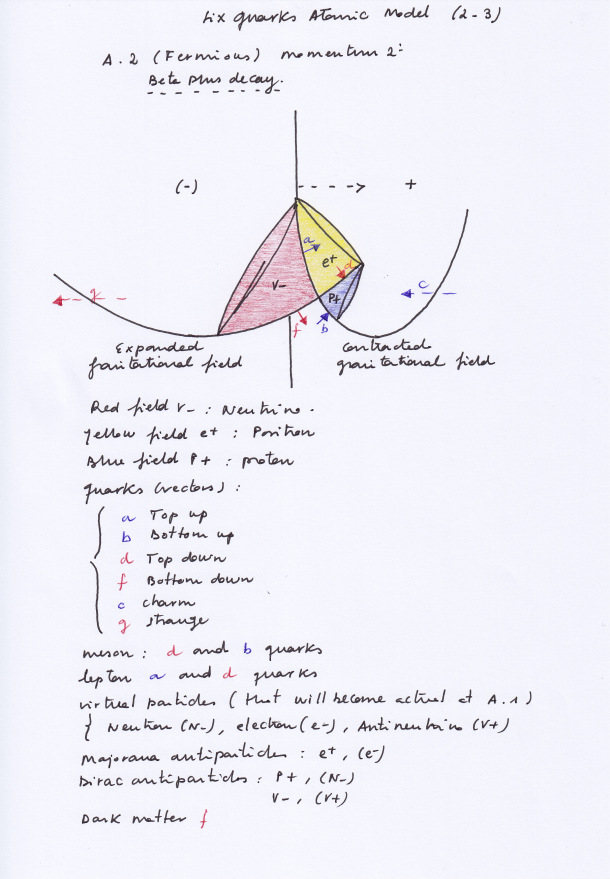
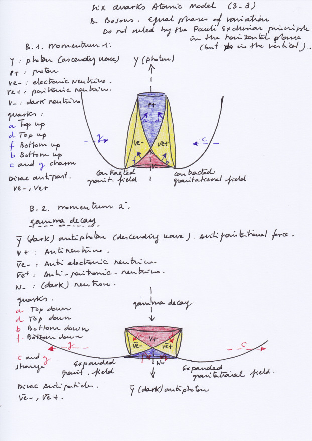
When it comes to 3D diagrams, the drawing I created some years ago for an alternative atomic model would be also related to these issues (and with the Lobachevsky imaginary geometry, that to me is not the same than the hyperbolic or curved geometry).
This alternative atomic is formed by at least two intersected concave fields varying periodically with the same or opposite phase, which create in their intersection four new subfields. Those subfields that form the atomic nucleus of this at list binary system, are a combination of the two intersected fields that created them and their behaviour and physical properties depend on the interaction of those periodically variable intersecting fields.
 .
.
If I have time I will also research about fuchsians equations and monodrom groups, that it seems are also related to these same subjects I mentioned on this post.
I’d also like to reseach about the work of Victor Puisexux that I feel is very closed to these kind of ideas, and later mathematicians as Sophus Lie, etc.
I think our mathematicians are speaking about almost the same or very similar kind of structures with very different terms, but they are not aware because of the absolute abstraction they are involved by. It would be as if many musical composers were writing a song for different instruments and none of them were aware that they are creating the same melody because no one has never listened to that music. When it comes to physics things have become even worse, because, with a music that nobody has ever listened to, they described the atomic nucleolus that no one had never seen.
Titanic efforts of intuition have been needed between mathematicians because of the lack of a visual representation of these subjects, and at the same time, the lack of a visual representation has excluded from the scientific realm to all people who need to visualize things to understand them, those who need to understand before continuing learning instead of only memorizing a subject and to operate with some provided tools in an instrumental and empty way, those who are not will to manage with absolute abstractions and to abandon their reason and their reasonable common sense, those who have highly critic minds, those who are actual researchers.
Finally, I’m going to attach some other figures drawing step by step how to build the extensions I was speaking about. Those figures are not anything new at all, but it seems no one used them before to explain these subjects. Maybe some who ask them, why?

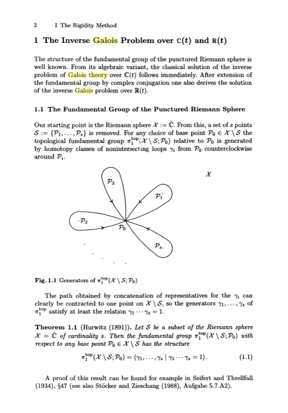
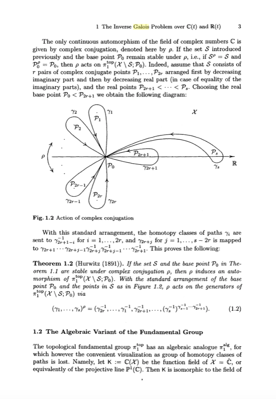
Between the books I took a look looking for visual representations of Gaslois groups, I only found these ones of professors Malle y Matzat, on their book “Inverse Galois Theory”:

Update Ag 7 2018:
With respect to the Riemann’s manifolds, I also found this article of Arkady Plotnitsky that explains it in a very clear and simple way: http://web.ics.purdue.edu/~plotnits/PDFs/Riemann.pdf
and https://web.ics.purdue.edu/~plotnits/PDFs/Manifolds.pdf
Have a good day
Note: The below ads are set and owned by WordPress as this is a free blog.

Escribe tu comentario