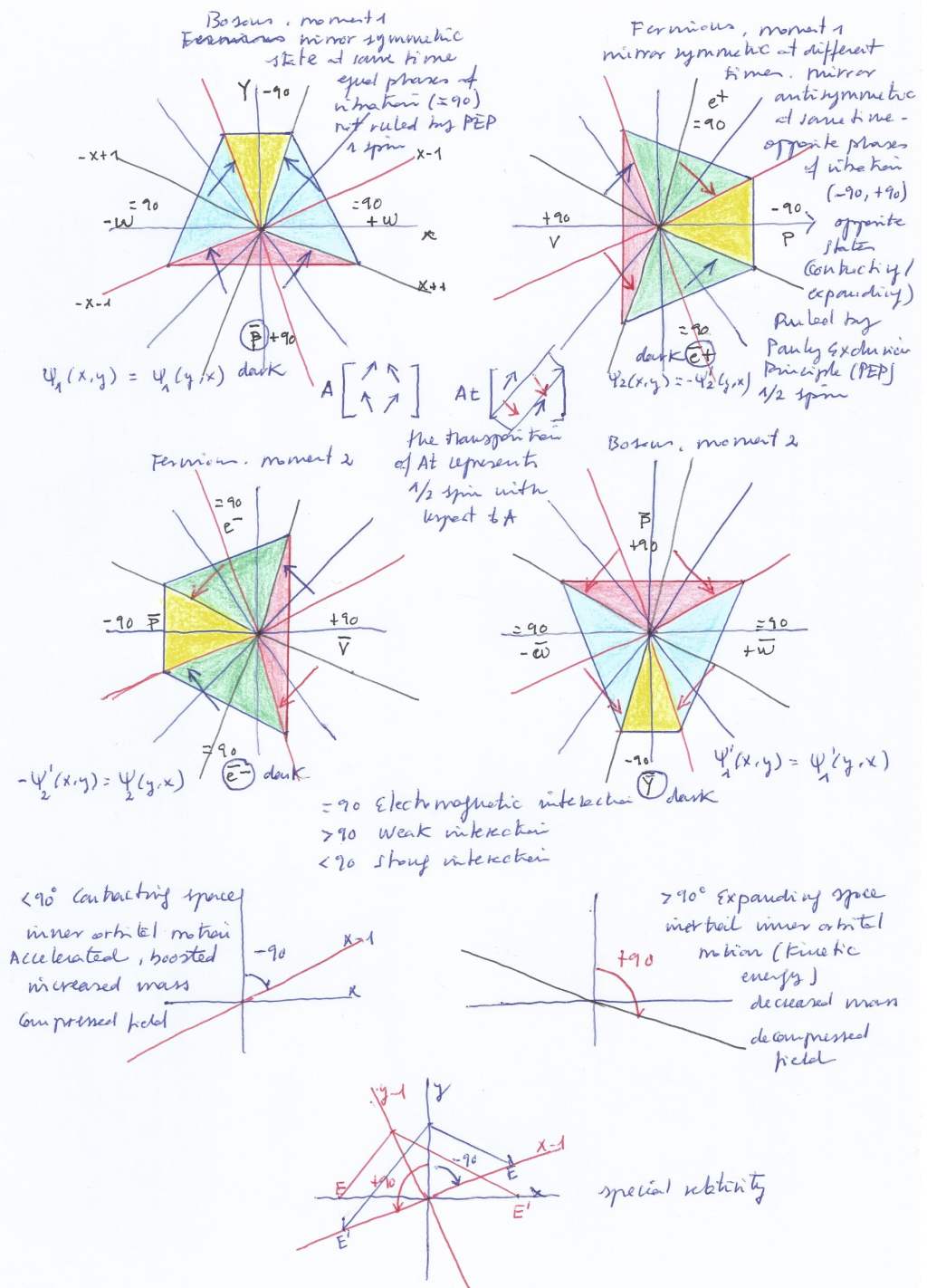
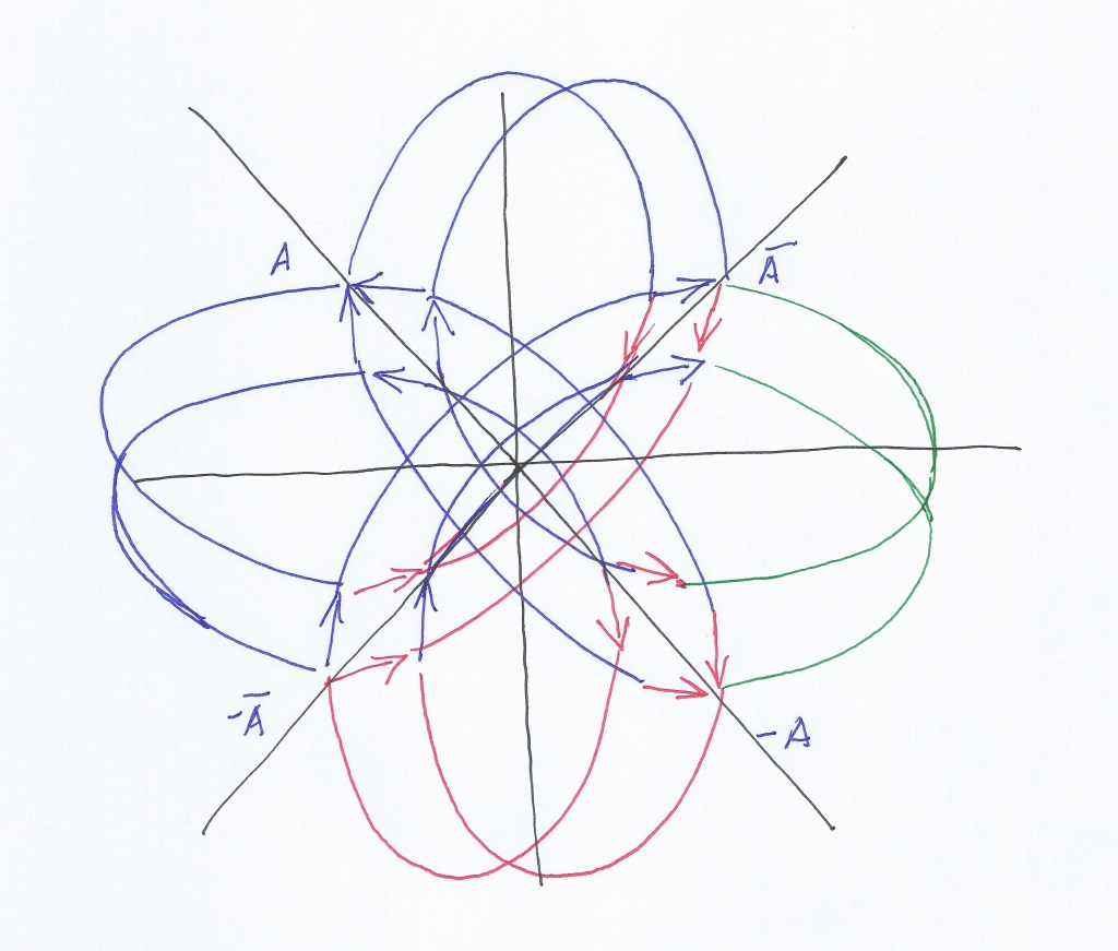
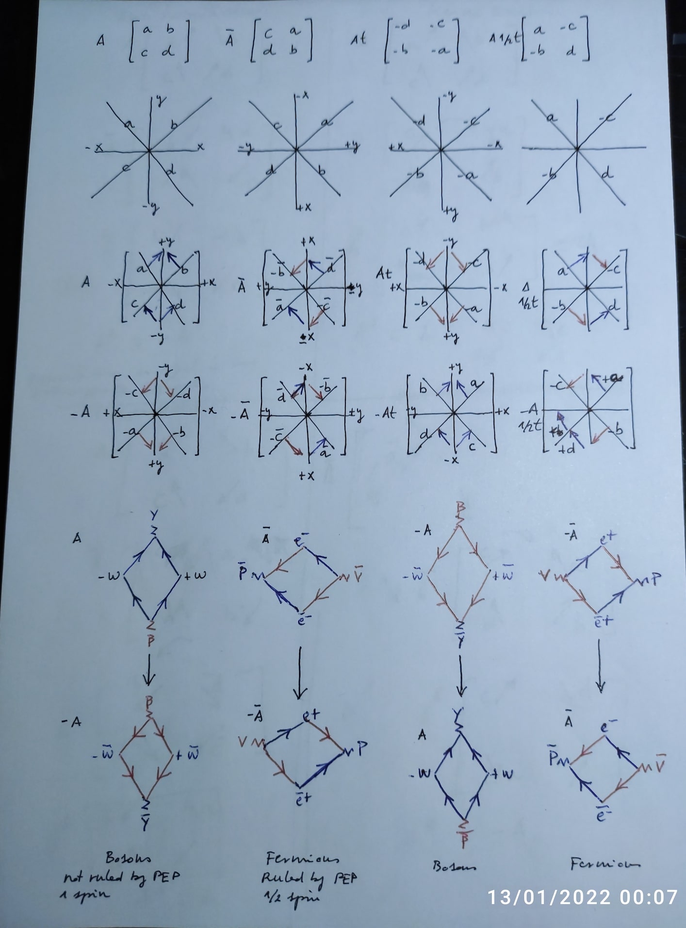
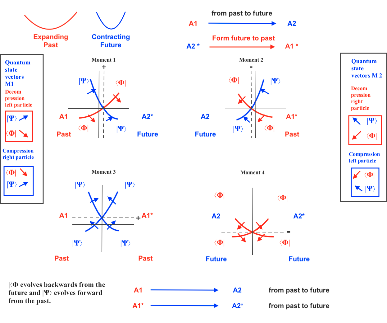
Let four positive vectors arrange on two rows and two columns being the elements of a 2×2 hamiltonian complex matrix. Rotate the vectors 90 degrees to obtain their complex conjugate; rotate 90 degrees the complex conjugate matrix to invert all the initial signs; and rotate the negative matrix to obtain their negative complex conjugate.

The blue color indicates the positive sign and the red color shows the negative sign of the vectors.
The operation of complex conjugation implies an actual transposition where the right diagonal vectors change their signs but it’s not possible to verify if they did or did not interchange their position.
Lets add a letter to each element to better distinguish them:

The four matrices that result after performing the 270 degrees rotation form 16 groups of symmetry taking the vectors in pairs, that are the ones we get when performing on the matrix A the operations of complex conjugation, transposition and inversion.
The matrix A can be considered as a second degree equation that provides different solutions equal to zero:
The square equation: A + Acc + (-A) + (-Acc) = 0

And the complex conjugate square equation: Acc + (-A) + (-Acc) + A = 0

(We could also add two more solutions starting by the negative matrices).
But we can also consider separately the non complex conjugate and the complex conjugate equations of degree 1:
The equation by A + (-A) = 0

And its complex conjugate equation Acc. + (-Acc.) = 0

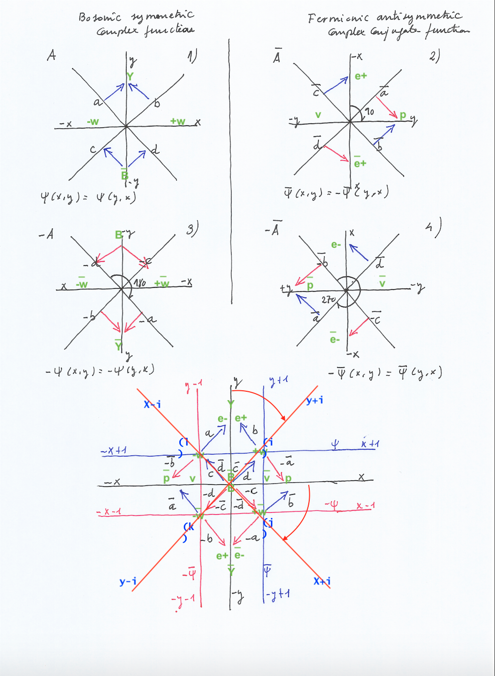
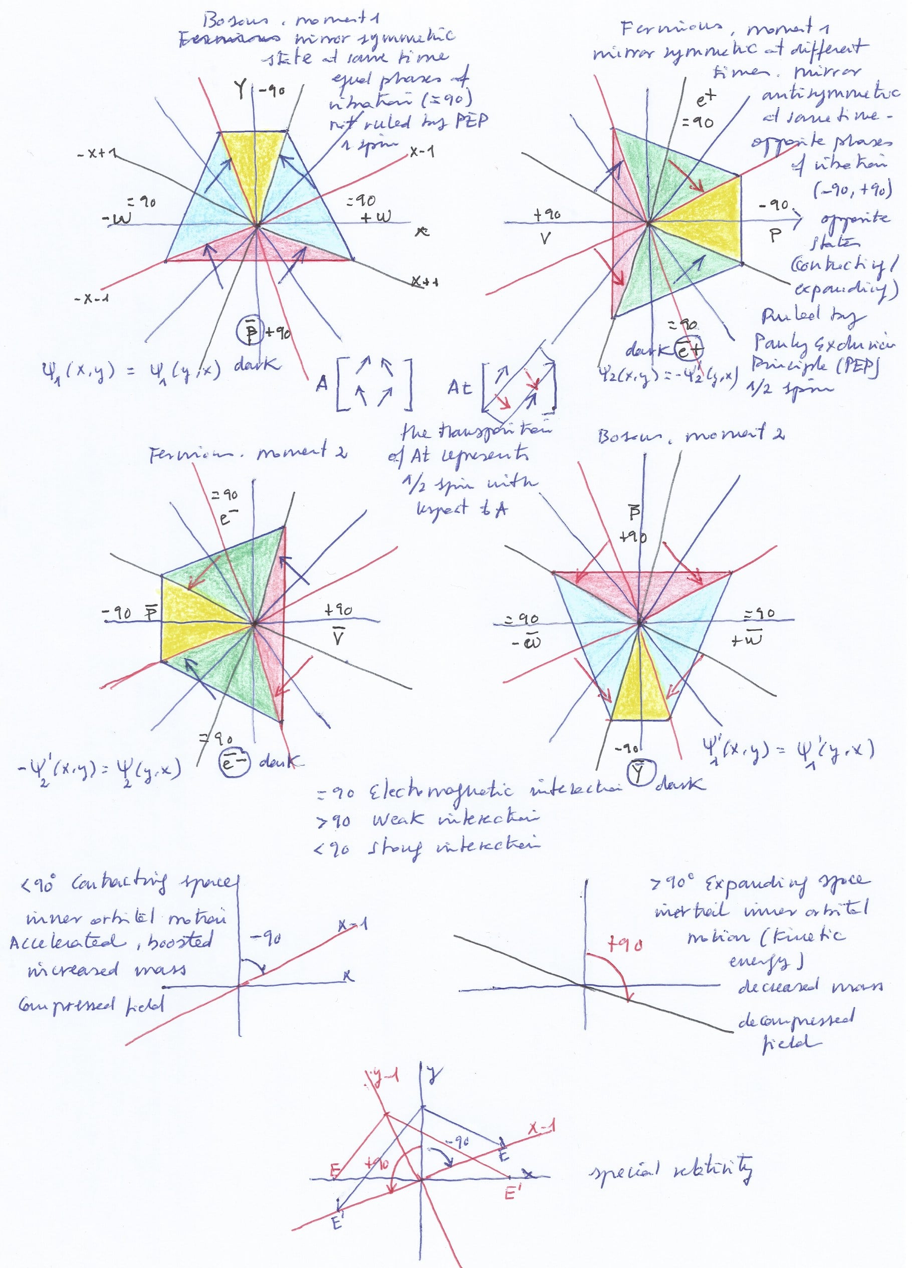
Considering first the normal (non complex conjugate) matrices that would form the 1 degree equation, we can also represent it as function where the + and – limits of its variations are given by the positions of the vectors of A and -A.
For example, if A and -A are related to the variations of a space that contacts and expands periodically, A would represent the moment where the space has its highest contraction, and -A the moment where the space reaches its highest expansion.
But as each matrix can be divided in two equal columns, we can think about each column as a transversal space that contracts or expands. And in this sense, we can deduce by the symmetric position of all vectors of A, that the left and right spaces will be mirror symmetric at the same moment given by A.
When all the vectors rotate becoming negative in -A, we can say that the all the elements of the system have changed their sign, the system will have an integer spin.
The left and right transversal spaces can be interchanged by means of a 180 degree rotation and they will remain being mirror symmetric. So it can be said that the system is symmetric under the interchange of the spaces.

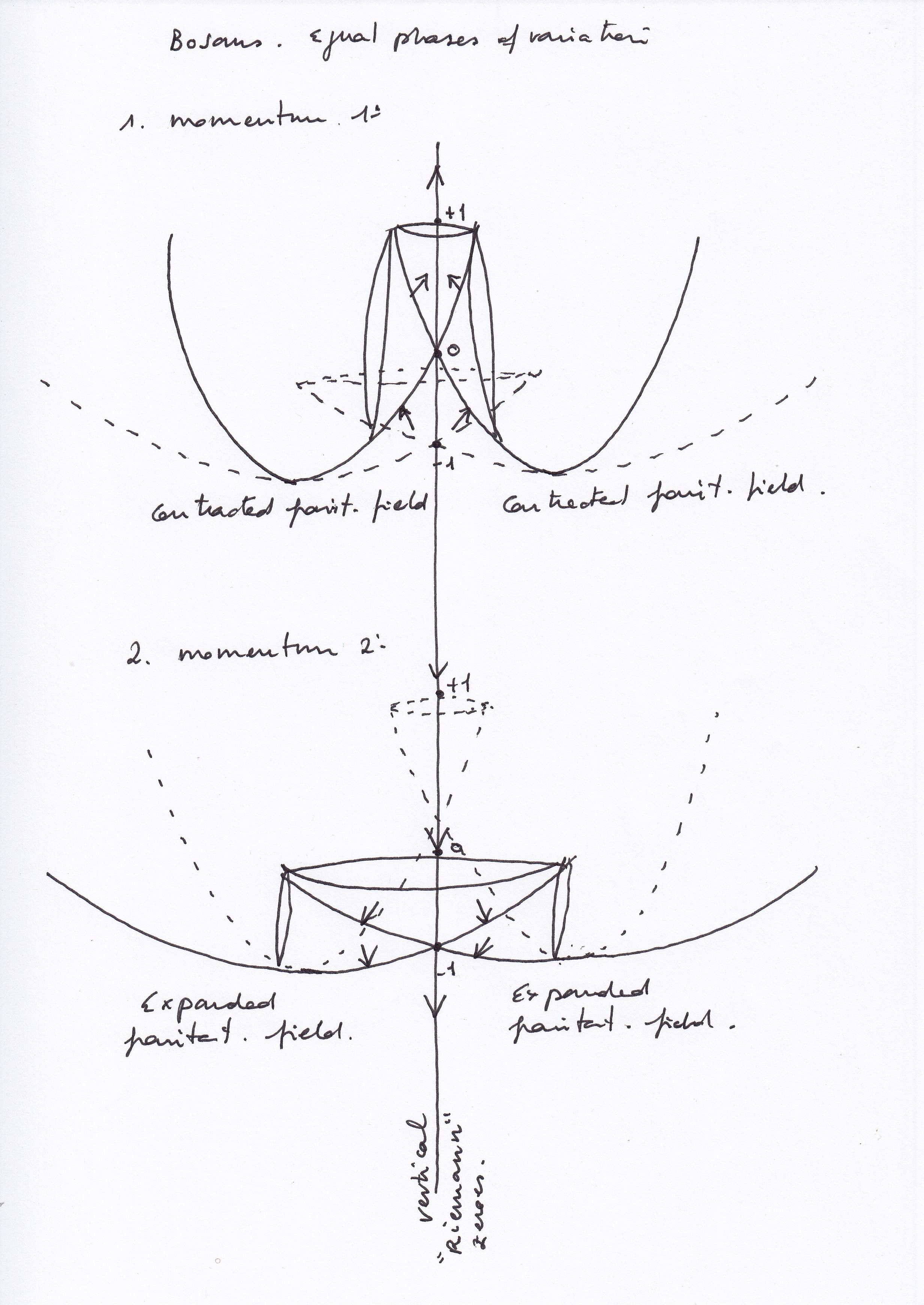
This function has then the same characteristics that a bosonic functions, where the left and right spaces will not be ruled by the Pauli Exclusion Principle; being identical, and being located at opposite places with respect a center of symmetry, they both simultaneously have the same status of expansion or contraction. Their phases of variation are symmetric.

In the case of the bosonic function, the orthogonal spaces – being in the bosonic system, follow opposite phase, we will see it later.
Now, lets see the complex conjugate function of 1 degree:
We can see on the above diagram that can be thought as a matrix, or a function with two particles or a system of spaces that form a nucleus, that the variation of the transversal spaces follow opposite phases, when the left space expands the right one contracts and vice versa. They are mirror antisymmetric spaces.
The status of A complex conjugate is reached when rotating A 90 degrees, and by doing that we see that two vectors changed their sign becoming negative. So, here we can say that only half part of the system have changed their spin. in this sense we can say this complex conjugate system has -1/2 spin in the case of A c. conjugate, and +1/2 in the case of -A c. conjugate (that changed the sign of half of the vectors becoming positive with respect to -A).
If we interchanged the left and right transversal spaces we would detect they have different quantum states. We use this term to refer to the status of being contracting or expanding and the physical properties (inner kinetic orbital velocities, energy, mass) and effect (forces of pressure).

So the phases of variation of the left and right spaces will be antisymmetric. In this sense they can be considered as fermionic spaces ruled by the Pauli Exclusion principle: the left and right spaces cannot be both expanding (or both contracting) at the same moment.
We will assign later specific names to those fermionic of bosonic spaces.
Now let’s see the square equation and its related matrices and functions and if they could describe different physical effects in the properties and behaves of the fermionic and bosonic spaces that the separate fermionic or bosonic equations did not point out.
It’s important to notice that here we are going to intercalate the + c. conjugate matrix between the + and – non c. conjugate matrices A and -A, and the negative non conjugate matrix -A between the + and – c. conjugate matrices. That is actually the natural sequence given when rotating the matrix 270 degrees.
But to represent simultaneously the sequence of statuses and the spins and signs of the vectors, we need to represent a fictional space where 4 past, present and future events simultaneously concur.
That is an «imaginary» multi time dimensional space.
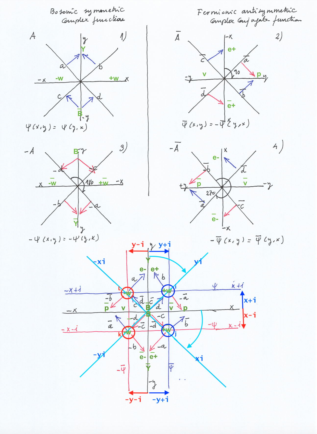

You can see all the status and vectors given by A, Acc. -A, -Acc. concurring simultaneously on the above diagram.
You can see there are additional X and Y coordinates above and below X, and at the left and right sides of Y. There are only two Z coordinates that here are named y=i, x+i, y-i, x-i.
The X Y coordinates are the real coordinates of the system; the y+i and x+i coordinates are the imaginary coordinates of the system. And the additional (displaced) X and Y coordinates are the location that the imaginary points would have on the real coordinates if they were not fixed.
The y+i coordinate is a Y coordinate rotated to the right 45 degrees and the x+i coordinate is an X coordinate rotated to the right 45 degrees. (We could also consider them as Z coordinates rotated 90 degrees).
The imaginary Y+i and X+i will be the real coordinates for a space whose central axis is rotated 45 degrees.
The fact that the real X and Y coordinates remain fixed while the Y+i and X+i coordinates rotate through time, lets us introduce the description of the movement on the real space, but also the description of the variation of the real space itself that would expand on the X+1 and Y-1 coordinates and would contract X-1 and Y+1 coordinates.
The diagram is a flat plane figure, but in this previously mentioned sense it seems to indicate a precession movement of the system while rotating 360 degrees around its central axis.
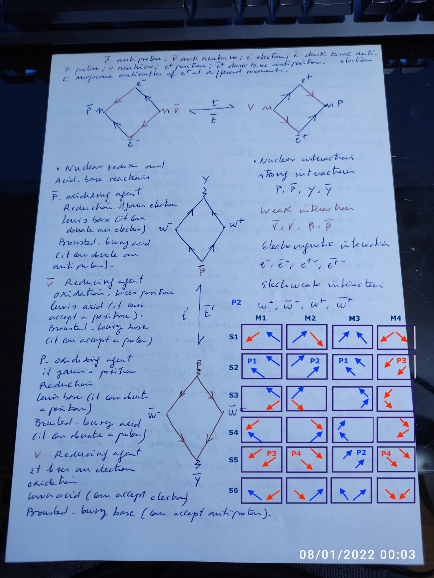
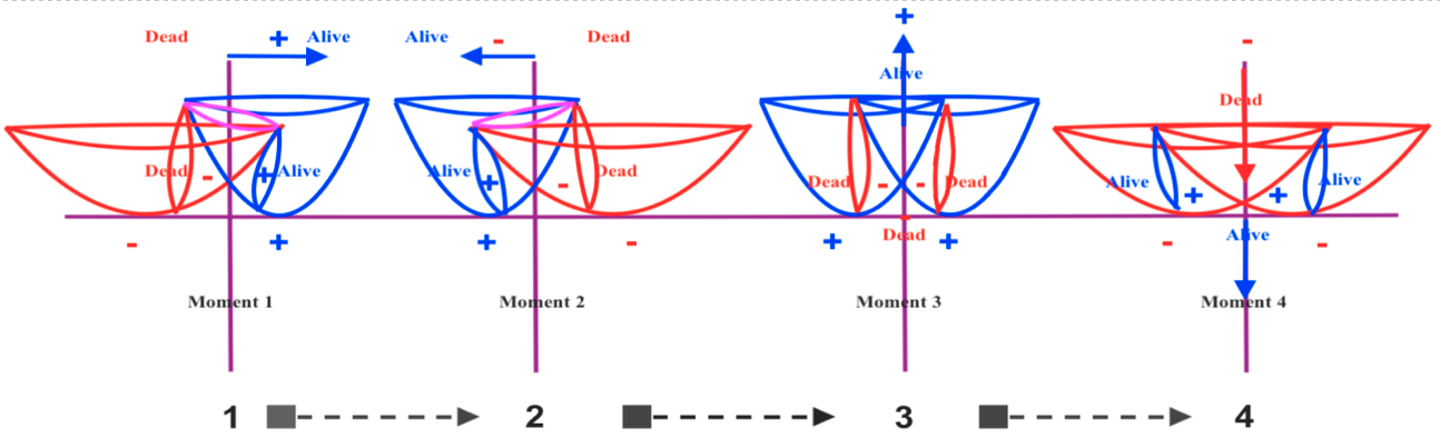
It’s also interesting to see how the two bosonic particles represented by -W and +W and their mirror symmetric antiparticles are placed on the four imaginary points of the system, while all the fermionic particles are placed on the real axes;
e- electron, e- antieclectron, e+ positron, e+ antipositron, p proton, p antiproton, v neutrino, v antineutrino.
The photon and the antiphoton will be placed as well on the real axis.
And the B decay and its anti B decay will be [placed on the cero point of the system.
It’s also interesting to see that from the point of view of the rotated XY imaginary coordinates, bosons are on the XY coordinates and fermions on the Z coordinates.
So, from the point of view of the real coordinates, fermions will be real and bosons imaginary; but from the relativistic point of view of the rotated XY imaginary coordinates, bosons will be real and fermions imaginary.
On the other hand, when it comes to fermions, the system and its energy moves towards right and left (electron and positron cannot be placed simultaneously place at the left and right sides because they are the sam Majorana antiparticle. Electron and anti electron, being different spaces having mirror symmetry would be Dirac antiparticles.
(Those particles related to a bottom down (negative) vector, as the anti electron or the antipositron, would be dark).
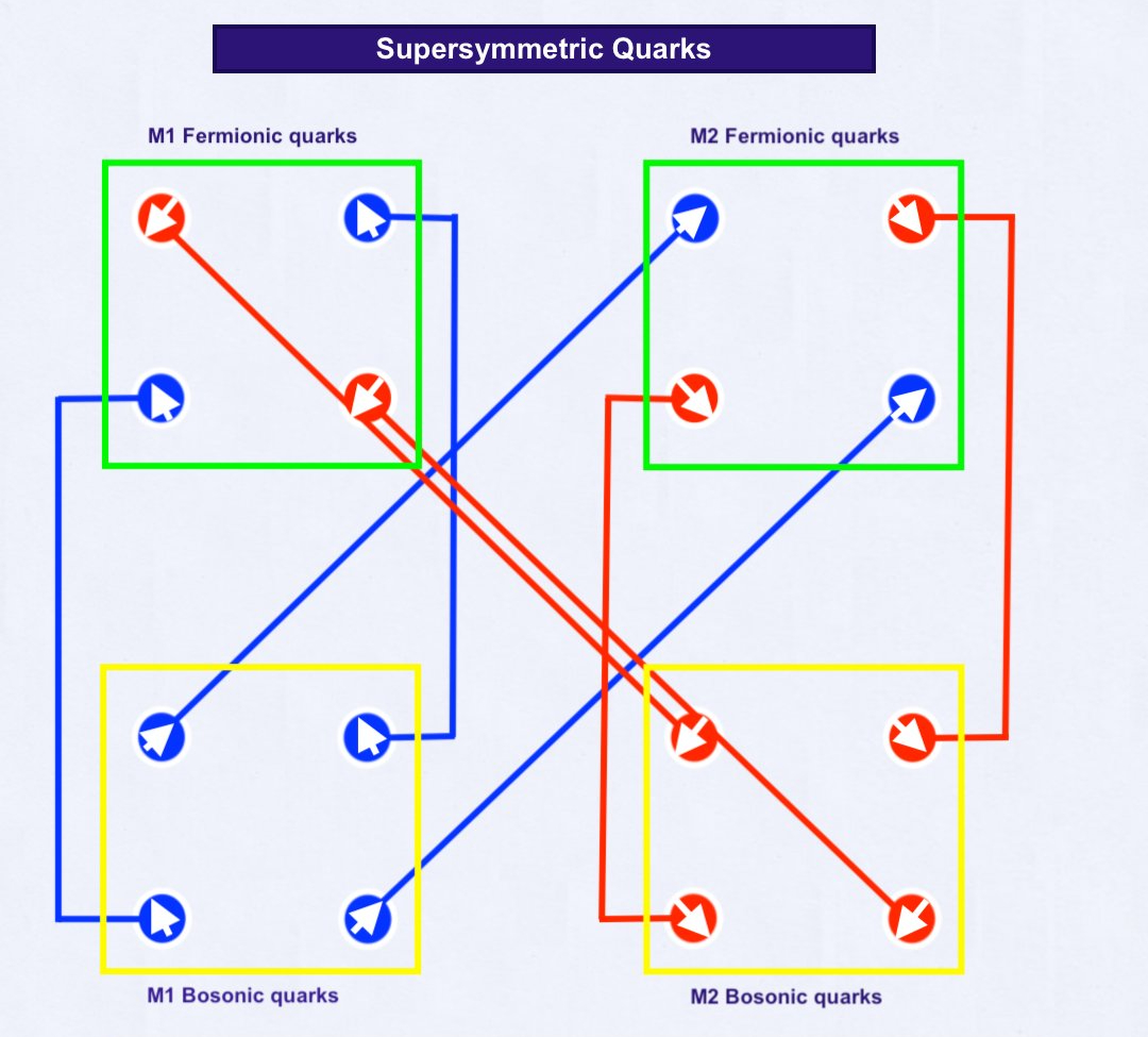
Watching simultaneously all the states, particles and vectors (that could be interpreted as force carriers or quarks in QCD) we see that the system is symmetric through time, that is to say, supersymmetric.
Mainstream models and theories like string theories have predicted the existence of supersymmetric particles that having symmetry through time would link the two kind of separate particles they have classify matter with: fermions and bosons.
To find out those supersymmetric particles is one of the main motives that larger and larger particle super accelerators are still being built. But supersymmetric particles have not been found so far.
But because physicists consider fermions and bosons as separate kind of particles or fields and expect to find additional particles to link them through time, seems to indicate that although the Schrodinger wave function is a second degree equation, and they are aware that the complex conjugate function describes fermions and the non complex conjugate describes bosons, for some reason that I don’t understand it seems they are not considering the combinatorial square function that naturally appears when rotating the 2×2 complex matrix 270 degrees.
I’m very curious about this question, as the combinatorial solution seems a pretty obvious option.
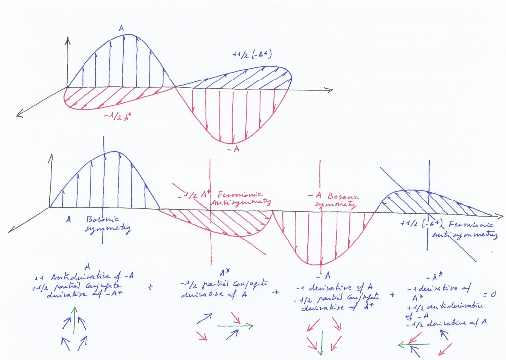
The Schrodinger equation is a «linear partial differential equation». And differential equations combine their derivatives. Maybe the Ac.c, -A, -Ac.c matrices we get when rotating A can be considered derivatives of A and the combination of A, Ac.c, -A, -Acc, by that order, is a differential equation.
I also read that there’s a type of matrix called «Jacobian» that collects all first order partial derivatives of a multivariate function.
I have to read about these things. But lets anticipate some ideas:
The A matrix is a complex matrix (each vector is on a z coordinate). A can also be interpreted as a function of two variables.
When rotating A matrix 90 degrees, we get its complex conjugate. If A were a complex function, its complex conjugate would be a first derivative.
When rotating the complex conjugate matrix 90 degrees, we when the -A matrix. in terms of a function, -A is the first derivative of Ac. conjugate and the second derivative of A.
Rotating -A 90 degrees we get -A c. conjugate, which would be the first derivative of -A, the second derivative of Ac. conjugate, and the third derivative of A.
Rotating -Ac. conjugate 90 degrees, we get the original A matrix. The forth derivative is then the original function in this case because by rotating the Z coordinates we are describing a circle.
But, the 2×2 matrix is not a four degree but a second degree equation. So we can think about Ac.c as the partial derivative of A, (only half of the vectors change their sign), -A as the complete derivative of A and partial derivative of Ac.c., etc. And we also can think about -Ac.c as the antiderivative, the integral, of -A, or even about the original A as the antiderivative of -Ac.c. because its a cyclic equation.

Now, we can combine the derivatives in a differential equation. And we can do it combining the derivatives in a complete differential equation (and in a complete complex conjugate differential equation) or in a partial equation (and in a complex conjugate partial differential equation).
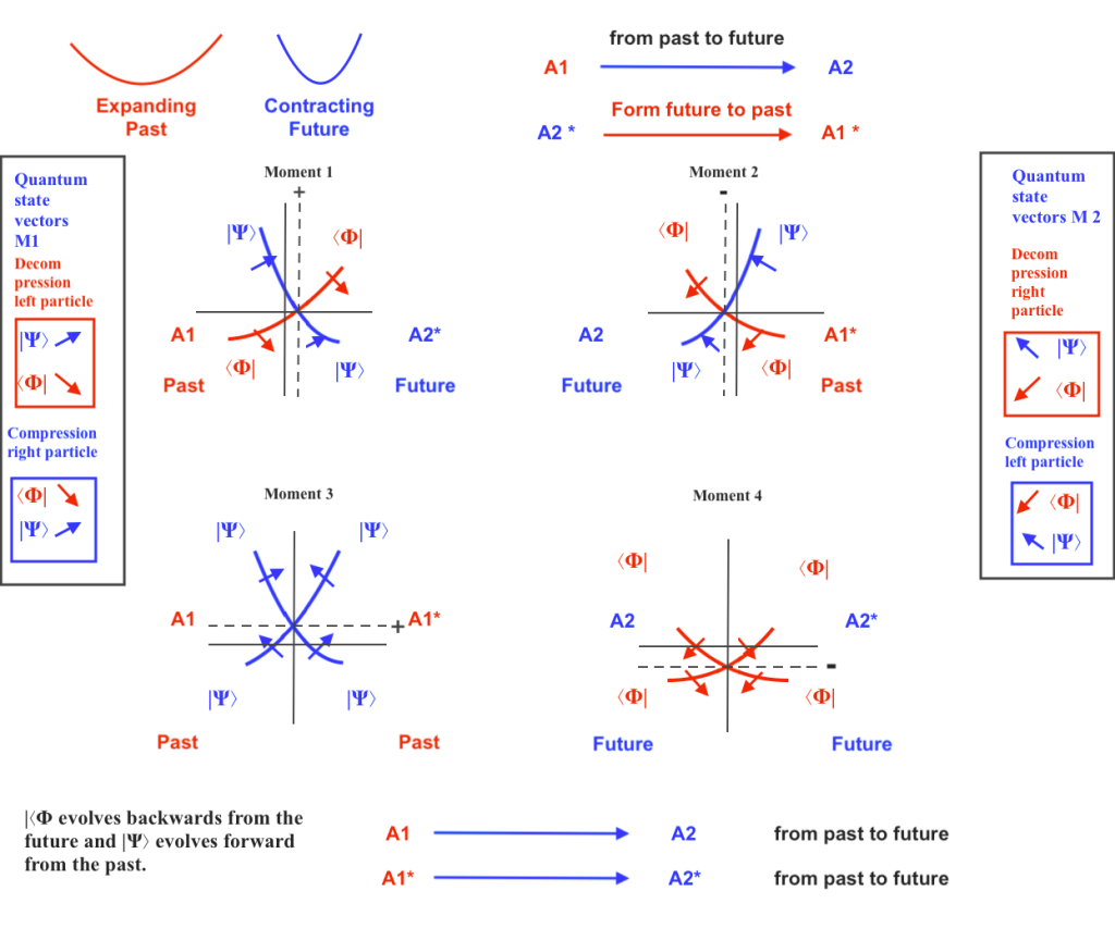
By combining A and -A we get a function the describes bosons. The left and right sides of -A the matrix (or of -A) matrix can be interchanged when rotating the system in a horizontal way 180 degrees. They are not ruled by the Pauli exclusion principle. They have integer spin because when rotating the matrix 180 degrees in an orthogonal way, all the vectors have changed their sign.
By combining the complex conjugate derivatives Ac.c and -Ac.c we get a function the describes fermions. The left and right sides of Ac.c matrix (or of -Ac.c) matrix are antisymmetric. They are ruled by the Pauli exclusion principle. When getting the derivative of A in Ac.c. only half of the system changes its sign (what it implies an actual transposition), and getting the derivative of -A only half of the vectors change their sign from negative to positive, so we can say the system in the -Ac.c. here the system has -1/2 and +1/2 spin.
Mainstream models consider fermions and bosons as different separate particles or spaces, as some supersymmetric type of additional particles that should link fermions and bosons are being looking for.
The Schrodinger equation is a partial differential equation. So it seems it’s does not combine the whole derivatives but a part of them: A, -A (or Ac.c, -Ac.c in its complex conjugate solution).
But it’s also possible to use a differential equation that combines its derivatives in the way described by rotating the matrix 270 degrees: A, Ac.c., -A, -Ac.c
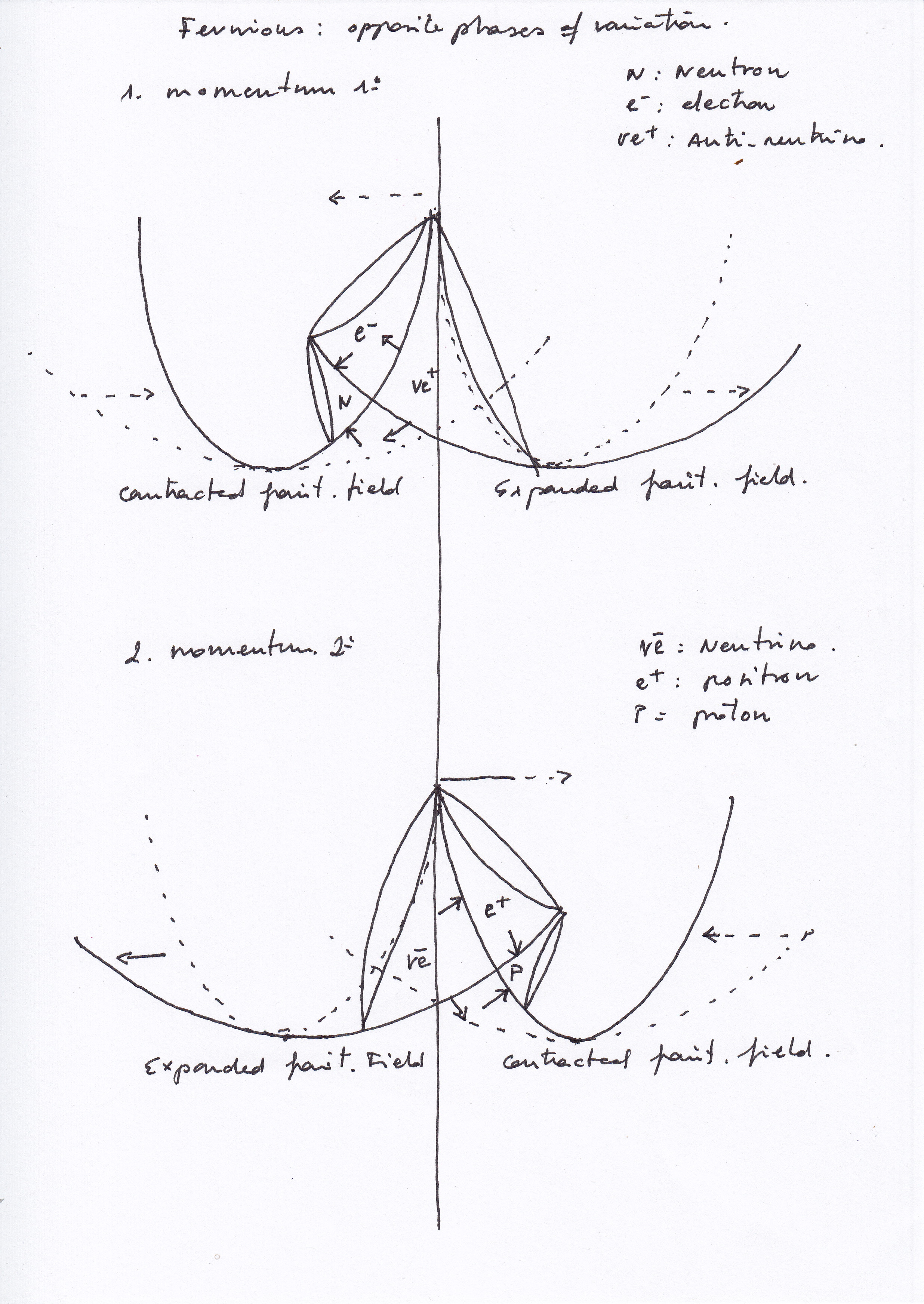
By means of that, we get the description of the bosonic and fermionic particles as 4 topological spaces that are transformed through time, acting as fermions or bosons, while the nucleus rotates, synchronising and desynchronising their phases of vibration.
If the Schrodinger equation is a partial differential equation, and it does not use the complex conjugate derivatives, if the atomic nucleus rotates, it’s going to leave out half part of the nucleus. To jump from the A equation to its second derivative -A, without considering the complex derivatives, if we are trying to describe something circular is like to suppose the atom is flat.
The function A is not integrated by its second degree derivative -A but by its first partial derivative Ac.conjugate and by the first partial derivative of -A that is -A c. conjugate.
And in the same sense, -A will integrate with the partial derivative of 1 degree of A that is Ac. conjugate and by the first partial derivative of -A that is -Ac. conjugate.
In that sense, -1/2 A c.conjugate integrates with A, + 1/2 A c. conjugate integrates with -A, and -1/2 -A c.conjugate integrates with A and +1/2 -A c.conjugate integrates with -A.

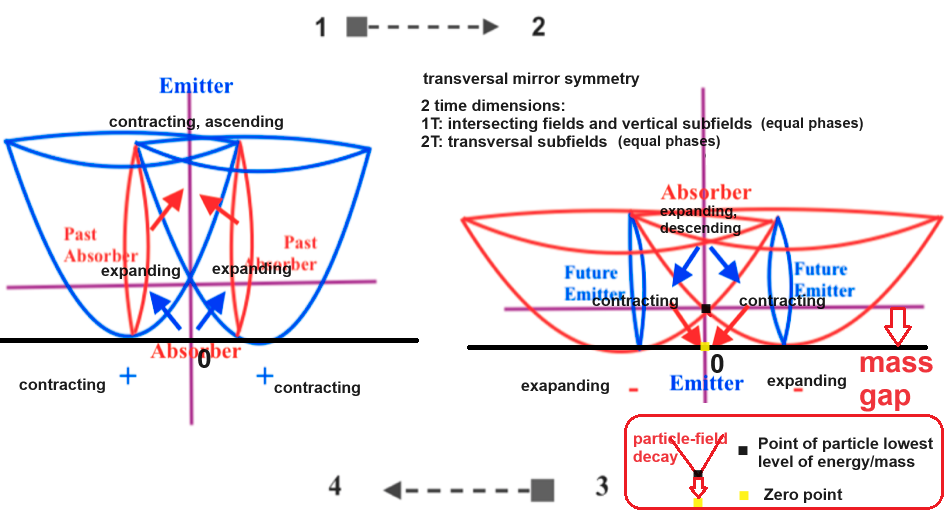
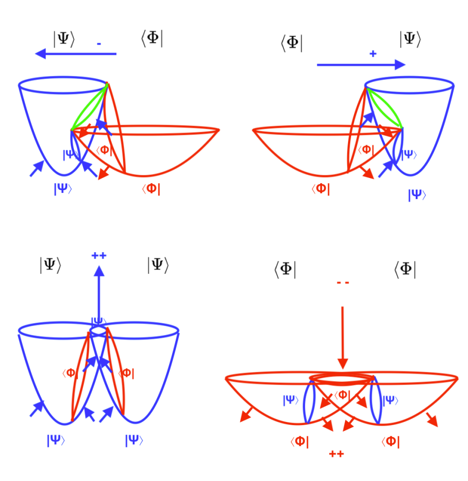
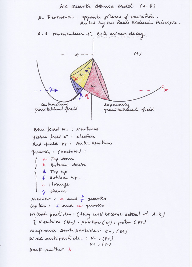
The atomic model I’ve been proposing on this blog is given by at least two intersecting spaces that vibrate with same or opposite phases, having a shared central nucleus of subspaces that would vibrate with same or opposite phases.
I presented it as two different systems, the bosonic and the fermionic, following the mirror symmetry and antisymmetry that the Pauly Exclusion Principle seems to underlay, pointing out that the same subspaces would act as fermions or bosons depending on the synchronisation and desynchronisation of their phases of vibration. And suggested that the vectors of force of the system (that I think would be quarks in QCD) that would be the forces of pressure or decompression caused by the intersecting spaces while expanding or contracting, would be supersymmetric.
According to the composite atomic model that I’m proposing on this blog, the the rotational nucleus model given by the 2×2 complex matrix would be shared by two intersecting spaces that vibrate with the same or opposite phase.
I already mentioned almost at the beginning of the development of the composite model that the nuclear particles could be related to imaginary numbers but by means of following the matrix operations I think the complex system about real and imaginary parts is clearer now.
Also I already mentioned that the Z coordinates could be interpreted as a Y or X displaced coordinates that create a new referential frame when the XY coordinates are fixed and we combined them with the rotated Z coordinates as if they were on a same plane, to describe a common space, given raise to the appearance of irrationality on the measure of the limited segments as the diagonal inside of the referential square of side 1, or when it comes to relate the perimeter of the circle and its diameter.
Have a nice week.
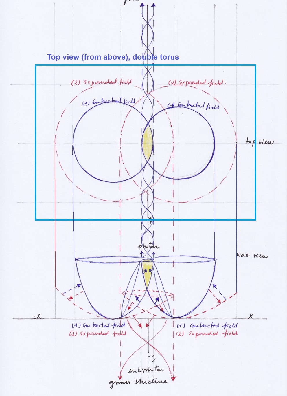
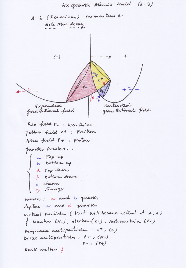
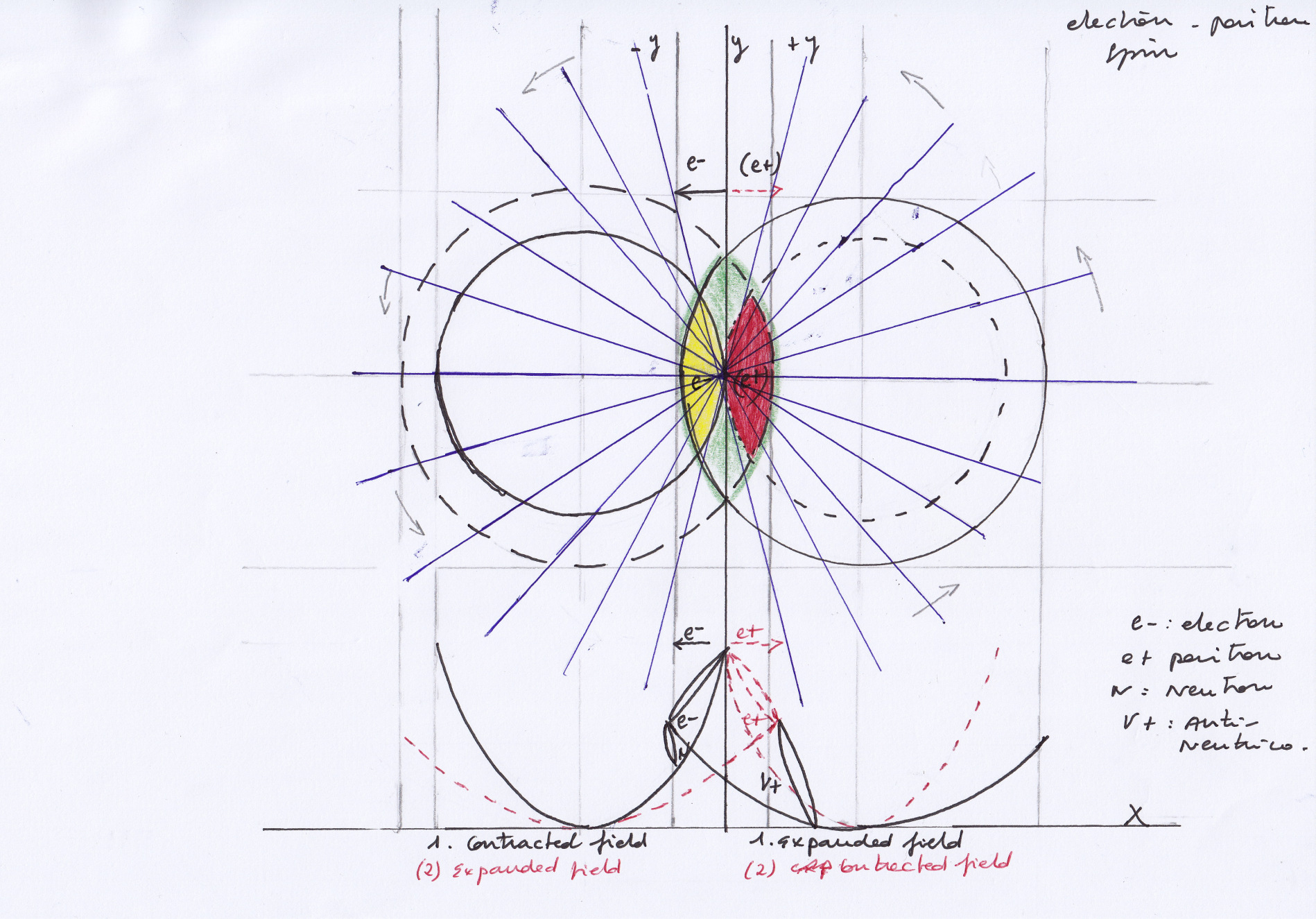
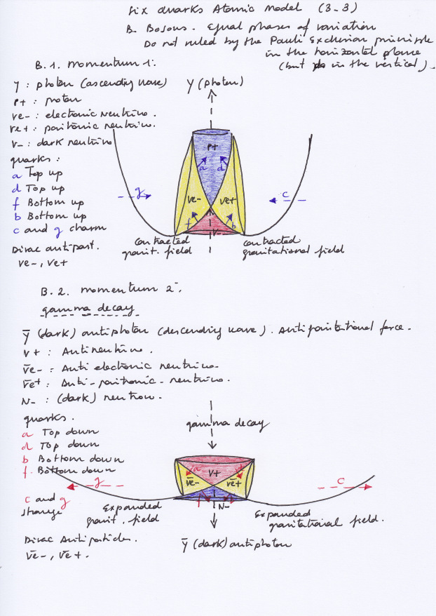
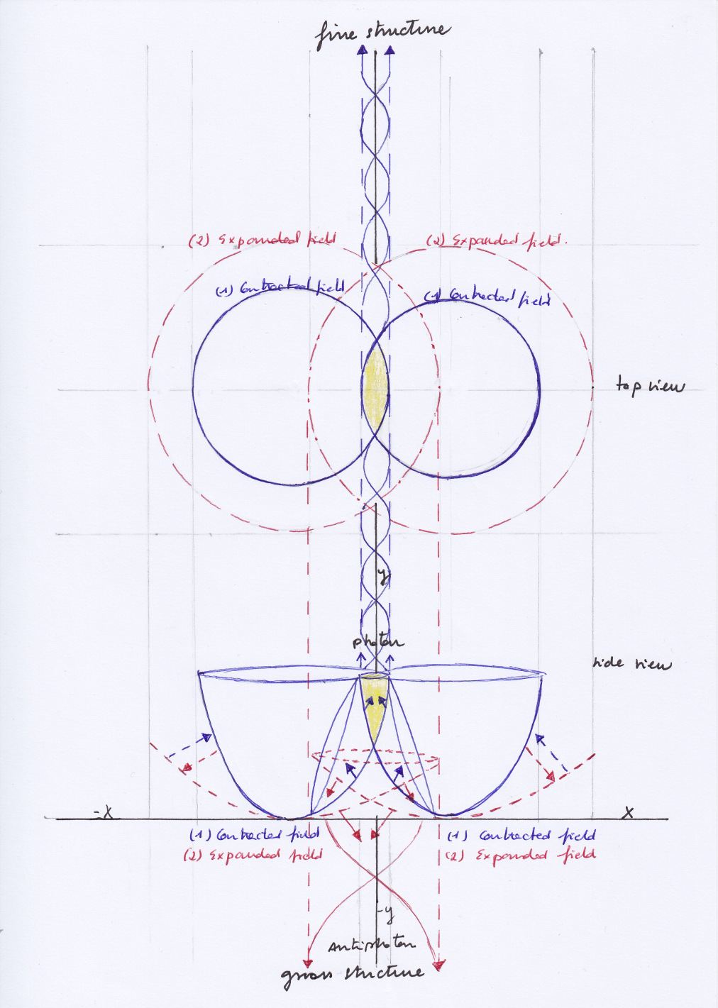
Some additional diagrams already posted related to the composite model:


The circle would also be a complex system, by the way.


Escribe tu comentario