*An updated version (En 9, 2024) of this post is provided in this pdf file:
.
Abstract: This paper introduces a non-conventional model within the framework of N=1 supersymmetric Yang-Mills theory [1], providing a visual explanation for the mass gap problem and the topological transformations of the supersymmetric atomic nucleus. The model is a supersymmetric topological manifold based on two intersecting fields that vibrate in either the same or opposite phases, forming four subfields. The bosonic or fermionic characteristics of these subfields are determined by the pushing forces generated by the intersecting fields’ negative or positive curvatures during their contraction or expansion.
The model employs a group of 2×2 complex rotational matrices of eigenvectors with eigenvalues 1 and –1 to represent these interactions and explores their implications for strong, weak, and electromagnetic interactions. It also introduces fractional derivatives to provide an interpretation of superposition and the exclusion principle in terms of mirror symmetry or anti-symmetry.
Keywords: SYM; mass gap; de Sitter vacuum; anti de Sitter space; zero-point energy; Sobolev interpolation; supersymmetry; supersymmetric quarks; topological gauge transformations; rotational gauge transformations; 2×2 rotational matrix; Hermitian; fractional derivatives; complex and conjugate Schrodinger equations; renormalization; mirror symmetry; antisymmetry; Pauly exclusion principle; superposition; entanglement; two-time dimensions; Calabi-Yau manifolds; elliptic fibrations; string theories; Ramond Ramond field; non-conformity; zero point energy; dark energy; Lobachevsky; Fourier; convolution; involution; Wick rotation; Minkowski, Tomita-Takesaki; modular matrices; polar decomposition; Langlands program; Langlands dual group; Cartan-Killing pairing.
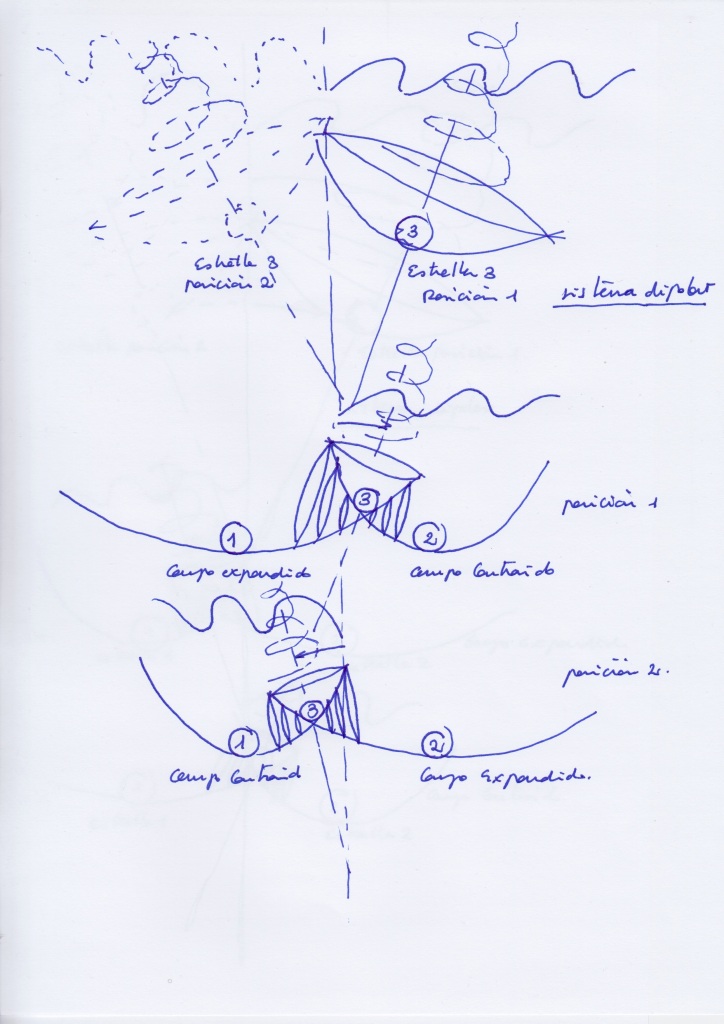
The model proposed in this unconventional paper is based on two intersecting fields vibrating with same or opposite phases that synchronize and desynchronize periodically. Their intertwinement gives rise to a composite manifold of 3 subfields in the concave side of the composite system and 1 subfield in its convex side.
The shape, mass, charge, inner kinetic energy, and spatial displacements of the 4 subfields will be determined by the pushing forces that the negative or positive curvatures of the intersecting fields generate while contracting or expanding respectively.
When the phases of vibration of the intersecting fields are opposite, the left and right-handed transversal subfields will be mirror symmetric at different times but mirror antisymmetric at the same time: when the left transversal subfield expands the right one will contract and conversely. The top vertical subfield will move right to left, getting a negative sign, or left to right, getting a positive sign, towards the side of the intersecting field that contracts; moving in a pendular way left or right, this subfield will be its own anti-subfield at different times.
The mirror transversal subfields are characterized by an antiphase relationship with each other, yet each of them maintains phase coherence with the intersecting space that encompasses it.”
Owing to their mirror anti-symmetry, the states of the left and right transversal subfields are mutually exclusive: when the left transversal subfield contracts, thereby increasing its density and inner kinetic energy, the right-handed transversal subfield will expand, leading to a decrease ins density and inner kinetic energy. In this sense, their states can be said to be governed by an “Exclusive” principle.
The opposite states of the left and right transversal subfields are not superposed because they are different spaces that reflect each other with a delay of time.
Within the framework of a dual composite system such as the one proposed in this model, both “superposition” and “exclusion” must be interpreted in terms of mirror symmetry or anti-symmetry.
In contrast, when the phases of vibration of the intersecting fields are equal, the transversal subfields will exhibit mirror symmetry simultaneously. Their states will be “entangled”. And, although they share the same phase, they will exhibit a phase opposition relative to the intersecting fields.
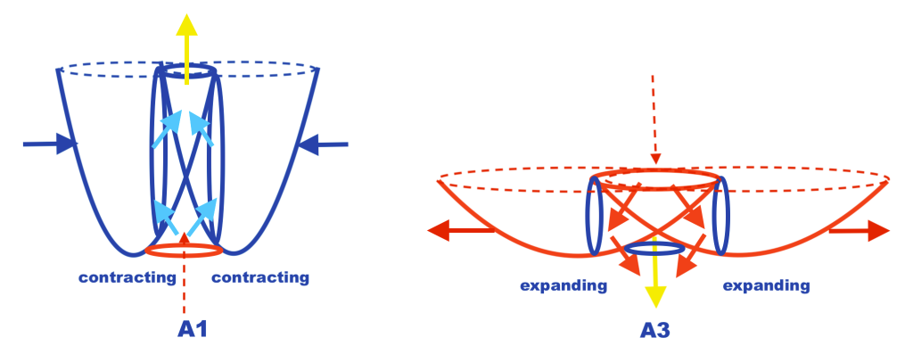
Once the system exhibits mirror symmetry, the top vertical subspace aligns with the phase of the intersecting fields: when both intersecting fields contract, the top vertical subfield also contracts, ascending upwards while emitting a pulsating force. Subsequently, when both intersecting fields expand, the previously ascending subfield decays while expanding. When such a decay occurs, an inverted pushing force is generated on the convex side of the system by the positive curvatures of the expanding intersecting fields.
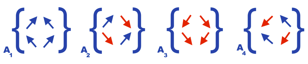
The pushing forces created by the contracting or expanding fields, with their inner negative curvature or their outer positive curvature, can be represented with 4 vectors.
Two vectors compressing a subfield imply a stronger force experienced by the subfield whose volume decreases while its density increases, and its inner orbital motion accelerates. The increased inner kinetic energy represents a greater bond that intertwines the intersecting fields in a stronger way.
Two vectors decompressing a subfield represent a weaker force experienced by the subfield, which expands in volume, decreases in density, and decelerates in inner kinetic energy. The decreased inner kinetic energy implies a weaker bond between the intersecting fields.
When considering the vibration of the intersecting fields, it’s important to note that the force of pressure that produces the convex or positive curvature of an expanding field will be weaker than the pushing force caused by the negative curvature of a contracting field, because the density of the expanding field will be lower than the density of the contracting field.
Alongside these strong and weak interactions, we are going to consider electromagnetic to the force caused by the vertical subspace when moving left or right in the antisymmetric system, and upwards or downwards in the symmetric system. The electric charge will have the pushing force that produces the displacements of those subfields. And we are going to consider gravitational the curvatures of the intersecting fields.
In addition to these strong and weak interactions, we will consider electromagnetic the force that the vertical subspace produces when moving left or right in the antisymmetric system and upwards or downwards in the symmetric system. The electric charge will be the pushing force that produces the displacements of those subfields. We will also consider as gravitational the curvatures of the intersecting fields.
The symmetric and antisymmetric manifolds can be considered either as two separate and independent systems, as two systems related by supersymmetric partners, or as two topological systems that are periodically transformed into each other by the synchronization or desynchronization of the phases of vibration of the intersecting fields, forming a single supersymmetric manifold. Here we only consider the latter case.
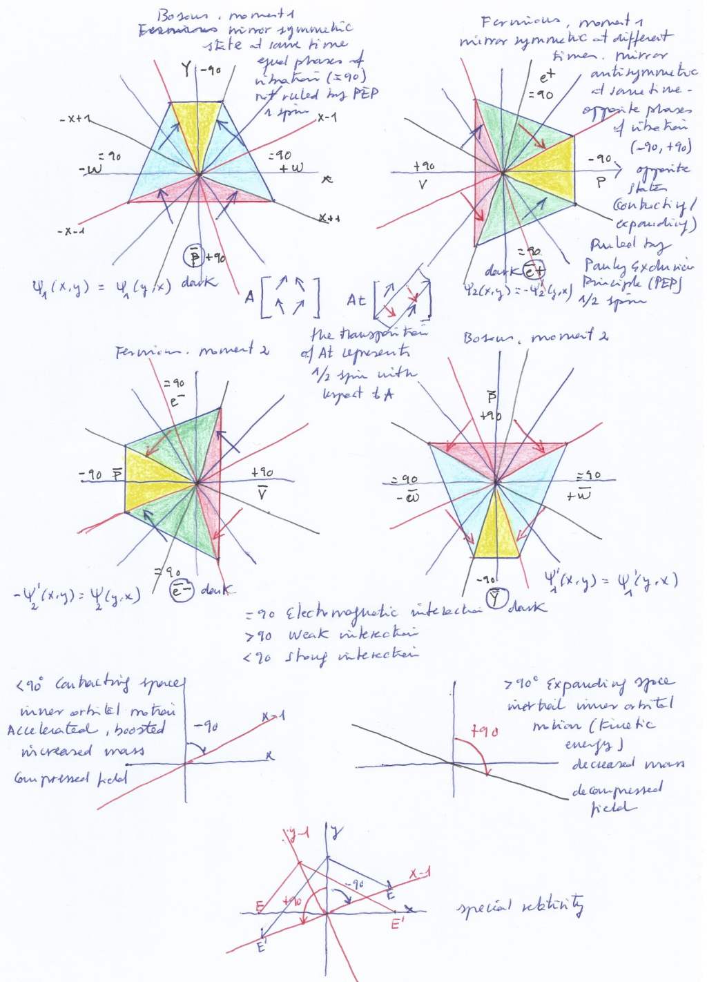
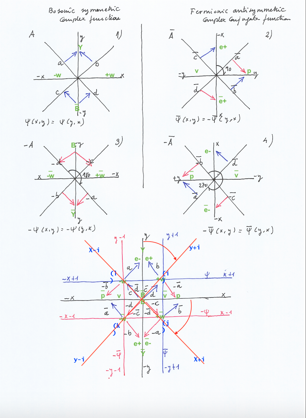
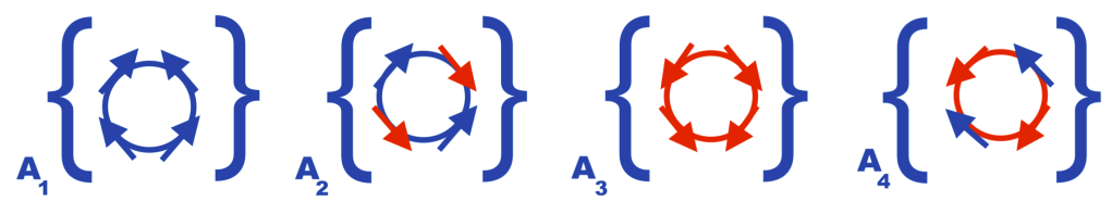
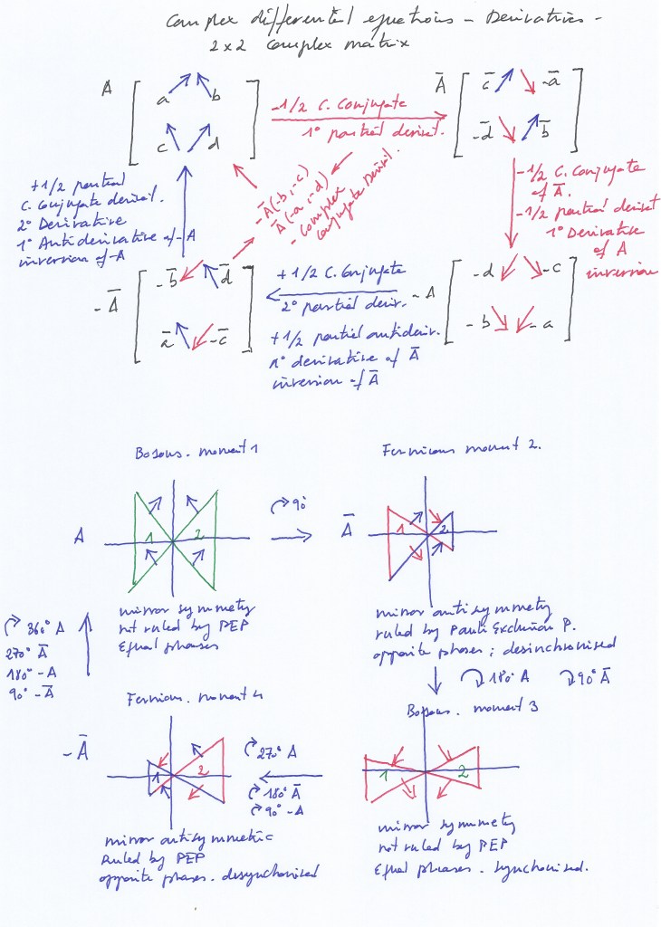
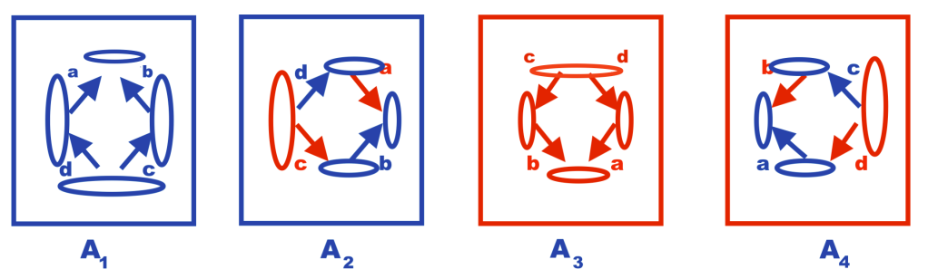
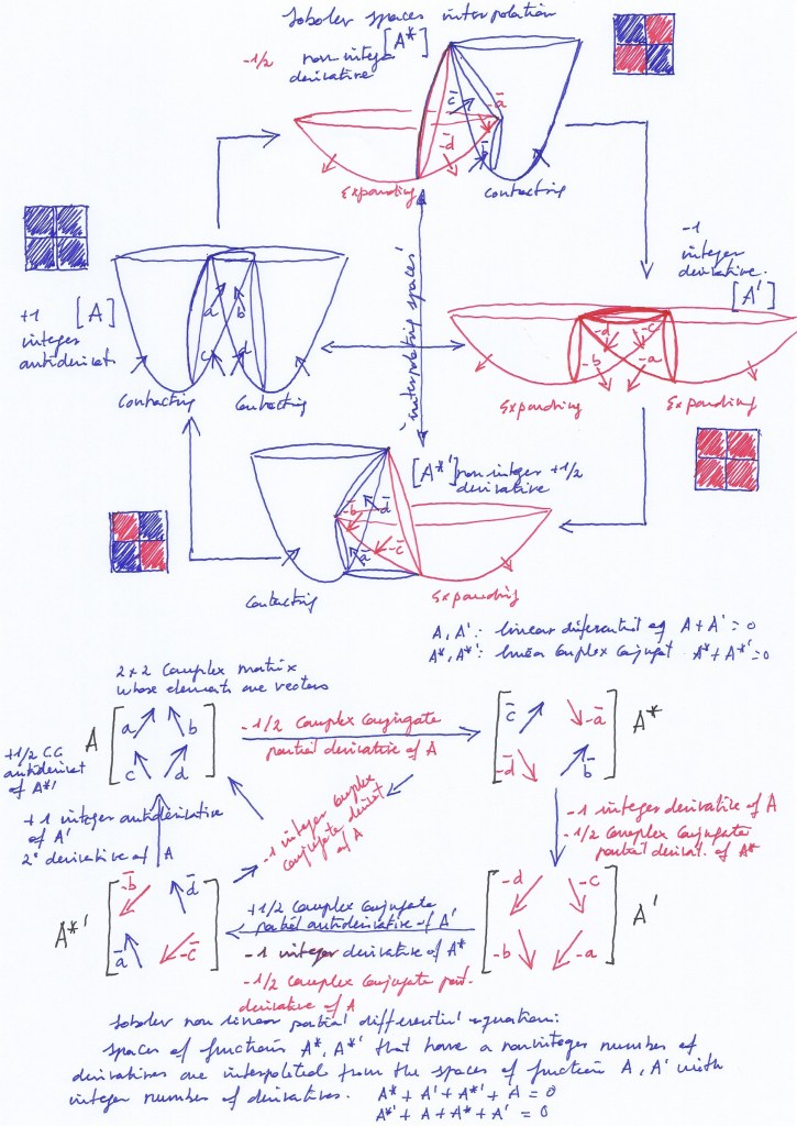
The system gets an additional complexity if it’s a rotational structure. Let’s examine the rotation of the system around its axis by means of a group of complex 2×2 rotational matrices with a 90-degree rotation operator. The elements of the matrices are four eigenvectors, that is, vectors that can change their sign but remain invariant in direction.
The eigenvectors will have an eigenvalue equal to 1 or –1.
The four vectors change their direction each time the whole plane rotates 90-degrees, but we can only distinguish a change in their position when their sign changes. A change in sign here implies a multiplication of the eigenvector magnitude by 1 or –1, being flipped or reflected across its origin, or being permuted 180 degrees.
The identity matrix A1 represents the position of the eigenvectors of the symmetric system when the two intersecting fields, in phase, contract simultaneously.
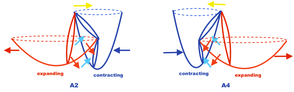
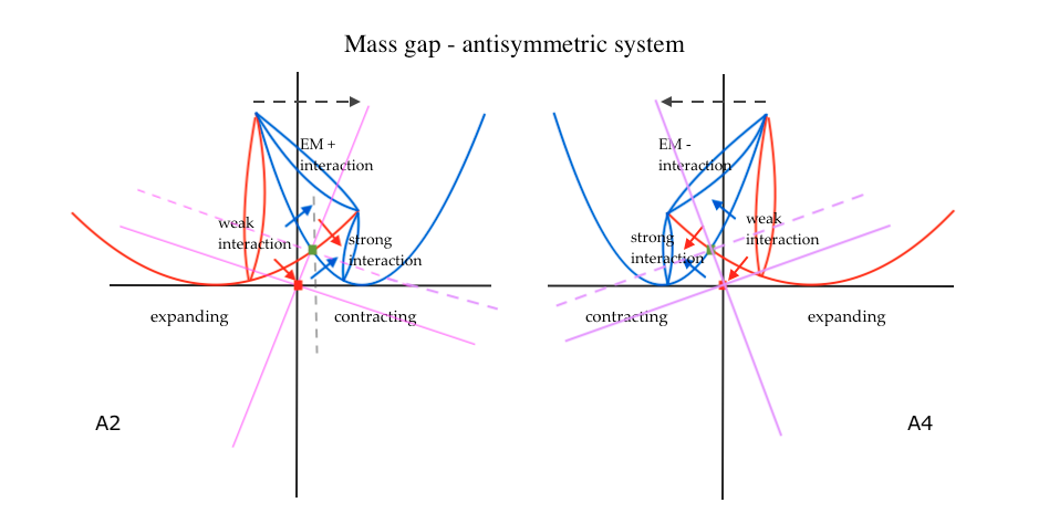
Rotating A1 by 90 degrees gives us the transpose matrix A2, whose eigenvectors represent the forces of pressure in the antisymmetric system when the left intersecting field expands and the right one contracts.
Rotating A2 by 90 degrees gives us the negative of A1, or A3. The A3 eigenvectors represent the forces of pressure in the symmetric system when the two intersecting fields expand with the same phase.
Rotating A3 by 90 degrees gives us the negative of A2, or A4. The A4 eigenvectors represent the forces of pressure in the antisymmetric system when the left intersecting field contracts and the right one expands.
Completing a 360-degree rotation by rotating A4 by 90 degrees gives us the inverse of A1, which represents the initial situation when both intersecting fields simultaneously contract.
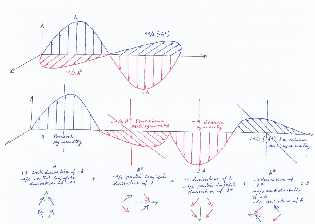
These operations can also be expressed in terms of differential equations, considering that those eigenvectors are tangent to a point of a unit circle of radius 1. The slope of the tangent vector will represent a derivative.
Each of the two sign-changing eigenvectors of A2, the top right and the bottom left eigenvectors, represents a derivative. A2 therefore contains a fractional number of derivatives: ½
If the rotated eigenvectors with changed signs represent the spin of the subfields in the antisymmetric system, the subfields represented by A2 will have a noninteger spin. In this case, their mirror counterparts will be governed by an exclusion principle.
A2 is a partial 1/2 conjugate solution of the complex matrix A1.
A3, the negative reflection of A1, represents an integer number of derivatives with respect to A1, 4/4=1, although it only encodes a fractional number of derivatives with respect to A2, the ones related to the upper left and bottom right eigenvectors with eigenvalue -1.
Therefore, to obtain the complete derivation of A1, it is necessary to rotate the matrix 90 degrees twice.
If the rotated eigenvectors with changed signs represent the spin of the subfields in the symmetric system, the subfields represented by A3 will have an integer spin. In this case, the transversal mirror symmetric subfields are not governed by an exclusion principle.
However, the top vertical subfield with integer spin and its reflection counterpart located at the convex side of the system will be ruled by an exclusion principle because when it contracts at the concave side of the manifold, its mirror reflection subfield will expand at the convex side.
For a detector placed in the concave side of the system, the mass and energy that occurs in the convex side of the intersection of the curved fields will be «dark» as directly undetectable.
A4 encodes two positive eigenvectors with eigenvalue +1. They are two antiderivatives with respect to A3. A4 also represents the negative of A2, and together they form a whole conjugate with respect to A1. Therefore, to obtain the complete conjugation of A1, it is necessary to rotate the matrix 90 degrees three times.
A1 represents the antiderivative of A3 and the half-antiderivative of A4. Therefore, to revert A1, the matrix must be rotated 90 degrees four times.
The rotational dynamic of the eigenvectors represented in this group of complex matrices, seems to imply that the smooth evolution of the symmetric system represented by A1 (when the intersecting fields contract) and A3 (when a moment later the intersecting fields expand), loses its continuity by being interpolated in between of A2 and A4.
In this sense, if the symmetric system is described by a complex ordinary differential equation and the antisymmetric system is described by the conjugate solution of the differential equation, then those separate equations can only describe the evolution and states of half of the system. In that case, the system may be incompletely described as discrete and could only be defined by statistical methods.
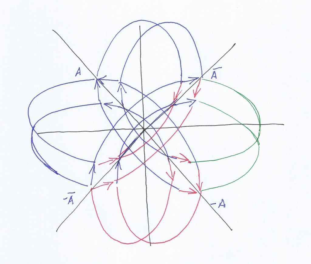
The next diagram represents the rotational eigenvectors in the rotational nucleus of subfields shared by the intersecting fields.
Although it is not clearly appreciable, the subfields in the picture change their shape while the 90-degree rotation is performed, as they contract or expand, move left or right, or ascend or descend, as a consequence of the vibration of the intersecting fields, while the system rotates.
However, we will discuss later the conformal or nonconformal nature of the model.
The interpolation between the symmetric and the antisymmetric systems may be related to Sobolev interpolations [2], where “spaces of functions that have a noninteger number of derivatives are interpolated from the spaces of functions with integer number of derivatives”.
Here, not only are the antisymmetric spaces that have a noninteger number of derivatives constructed from the symmetric spaces that have an integer number of derivatives, but also the symmetric spaces are constructed from the antisymmetric ones by means of a topological transformation.
The levels of energy of the four subfields can be inferred from the position of the vectors in the rotational matrix. In this sense, the supersymmetric group of matrices A1 , A2 , A3 , and A4 , with a 90 degree rotation operator, can represent the Hamiltonian of the supersymmetric system. The matrix A1 is Hermitian, as it is equal to its conjugate transpose. The conjugate of all the elements of A1 is obtained at A4 after three 90 degree rotations (adding the 1/2 conjugation of A2 and the 1/2 conjugation of A4 ). The transpose of A4 is A1 .
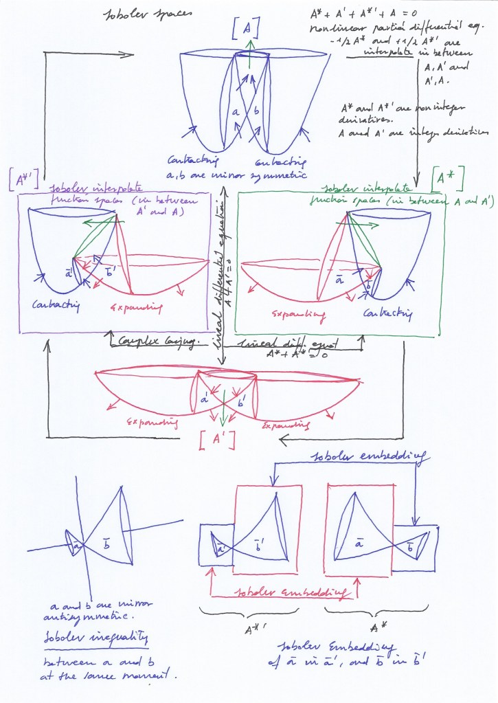
The combination of a complex ordinary function, represented by matrices A1 and A3, and a complex conjugate function, represented by matrices A2 and A4, can be also described as a convolution.
Adding the products of the four transformation matrices, their fractional derivatives or antiderivatives that represent partial conjugate functions, the identity matrix that represents the complex function is obtained.
The conjugate function is a conjugate harmonic function, as it is the conjugate partial derivative of a first-order complex ordinary function.
In the rotational context, the symmetric system of mirror subspaces (described by the complex ordinary function represented by matrices A1A3) becomes antisymmetric (in A2) when performing a partial conjugation (rotating A1 90 degrees) that generate transposition by means of a fractional differentiation.
Antisymmetry arises in the mirror system by introducing a change of phase in one of the sides of the reflection, while the other side keeps following the unchanged phase. That change of phase can occur by a gradual desynchronization, or suddenly, when a rotation occurs changing the sign of ½ eigenvectors or spinors.
The addition of the main and harmonic phases can be performed with a Fourier transform, obtaining a third combinatory frequency.
The symmetric and antisymmetric systems can also be described as two independent groups of cyclic eigenvectors that form two von Neumann algebras: an antisymmetric automorphic algebra and a symmetric automorphic algebra, which imply antisymmetric and symmetric mirror reflection algebras, respectively.
However, both independent algebras can be related by means of modular combinations, which, in the context of our rotational matrices, are the combinations of the transform matrices with fractional derivatives or antiderivatives.
Modular combinations of von Neumann algebras are studied by Tomita-Takesaki (TT) theory.
In TT theory two intersecting algebras form two shared “modular inclusions” (with + – “half sided” subalgebras) and a “modular intersection” (with an “integer sided” subalgebra).
The left and right half handed subalgebras will be the image of each other, when they are commutative, or they will not be their image when they are noncommutative. Mapping the modular inclusion to its reflection image, the left and right subalgebras will be the opposite image of each other (reverting their initial signs) if they are commutative; if they are noncommutative, the initial left sided subalgebra will be the image of the right sided mapped subalgebra, and the initial right handed subalgebra will be the image of the left sided mapped subalgebra.
TT theory decomposes a linear transformation into its modular building blocks, revealing the hidden automorphisms. Decomposing the bounded operator, it obtains the modular operator and the modular conjugation (or modular involution) which is a transformation that reverses the orientation, preserving distances and angles).
Translating the abstract algebraic terms to our present model, we can say that the two TT intersecting algebras represent our two intersecting fields vibrating with same or opposite phase. The half handed subalgebras (or “modular inclusions”) will be the transversal subfields of the nucleus shared by the intersecting fields, while the integer handed subalgebra (or “intersection inclusion”) will be our vertical subfield. In this context, we identify commutativity and noncommutativity with mirror symmetry and mirror antisymmetry respectively.
The bounded operator that is decomposed will be the 90 degrees rotational matrix; The modular building blocks are the set of matrices that are obtained when applying the operator. The modular operator will be the ½ partial conjugate A2 matrix; And the modular conjugation will be the conjugate matrix A4 (which forms the whole conjugation by adding the fractional conjugations ½+½). So, separating the conjugate matrix from the complex one the automorphism of the antisymmetric conjugate system is found.
The half sided algebras that form a modular inclusion are noncommutative, it means we are in the antisymmetric system where the left intersecting field contracts while the right one contracts and vice versa; in that system, the left transversal subfield will be the mirror symmetric image (it will be the mapped image) of the right transversal subfield when, later, the left intersecting field expands and the right one contracts. In that sense we are mapping here a past half handed algebra with its future image. A time delay exists between both algebras.
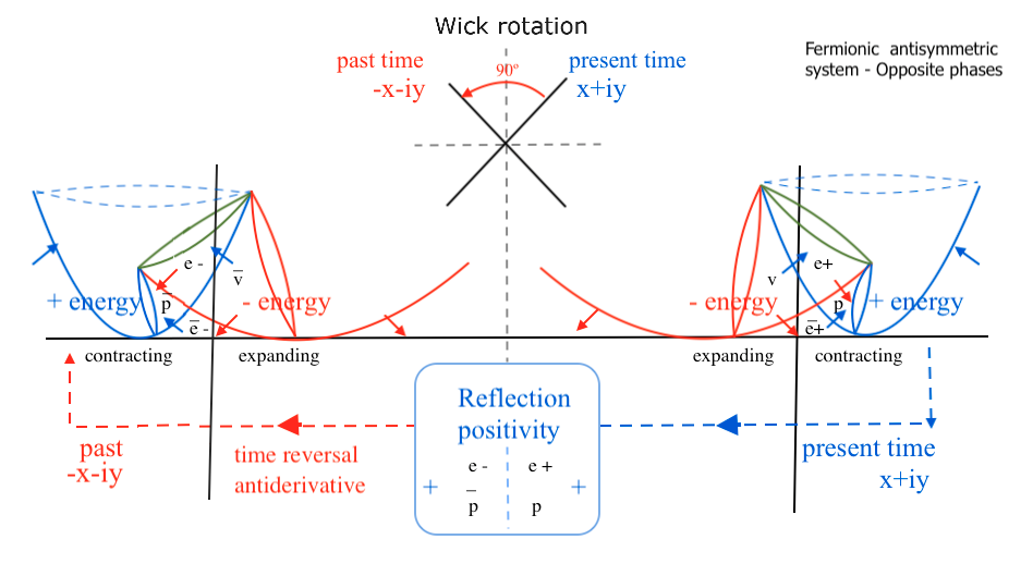
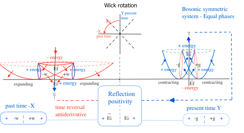
Related to this delay of time in the antisymmetric system, we can also mention a property that all unitary quantum field theories are expected to hold: “Reflection positivity” (RP). [3]
The positive increasing energy that appears on one side of the mirror system should be reflected as well in the other side. But in the context of the antisymmetric system, we find that positive energy of the contracting right transversal subfield is not simultaneously reflected in the expanding left transversal subfield, which has a negative energy.
Because of that, to obtain a positive energy reflected at the left side, making the sides of the system virtually symmetric, a time reverse operation will be needed.
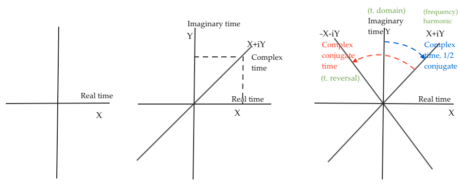
To see the positive energy reflected at the left side we will need to go back in time to the moment where the left transversal subfield was contracting having a positive energy. That operation is performed by a type of Wick rotation.
We can represent the main time phase of the symmetric system with the Y coordinate.
Performing from there a partial conjugation that involves a fractional derivative, the time coordinate rotates to the complex plane. At that moment the mirror system becomes antisymmetric as one side of the system keeps following the imaginary time of Y while the other side follows a harmonic phase.
A positive or negative time lag has been introduced.
To go back in time on side of the system is a way of virtually making the time phases symmetric again. To achieve that time reverse we make a reverse rotation of the complex time axis X+iY to complete a whole complex conjugation at –X –IY.
That time backwards rotation represents an antiderivative. (If it were forward it would represent a derivative).
When the time reverse has been symbolically completed, we will presence in the left side of the mirror system how the left subfield contracts having an increased positive energy; it is a past reflection of the future positive energy that there will be a moment later in right side. In this past time, at the right side of the system the right subfield will be expanding having a decreased negative energy.
When it comes to the symmetric system, positivity is reflected between the right and left transversal subfields at same time. In that sense, it’s not necessary to use the Wick operation to reverse time. Both left and right transversal subfields will be mirror reflection of each other at the same time.
However, in the case of the strong interaction in the symmetric system, when the contracting vertical subfield has an increased positive energy while ascending to emit a pushing force, it will be necessary to virtually visit a past moment to look for a previous state where positivity could be reflected. Going back in time, we will find that the vertical subfield is losing its energy while expanding and moving downwards. So, at that moment of time the vertical subfield will not display a positive energy.
Reflection positivity, however, can be found at that past moment in the convex side of the system of the two intersecting fields where an inverted subfield with a double positive curvature will be experiencing an increased energy. That inverted subfield can be mirroring related to the vertical subfield that in a future state will be ascending in the concave side of the system.
The missing reflection positivity in the concave side of the system in the strong interaction can be related to a mass gap problem when it comes to the weak interaction.
There will be a mass gap in the system when the two intersecting fields simultaneously expand, and the vertical subfield experiences a decay of energy.
This case represents the lowest possible energy of the subfield, which is always greater than 0 because the highest rate of expansion of the intersecting fields prevents them from having zero curvature.
The zero point of the vacuum where there is no energy and mass is placed at the point of intersection of the XY coordinates, and that point is never reached by the descending and expanding subfield that decays.
An “upper mass gap” would be referred to the highest possible mass of a particle in the strong interaction. Its limit would be given by the greatest rate of contraction of the intersecting spaces.
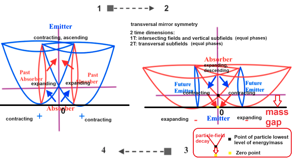
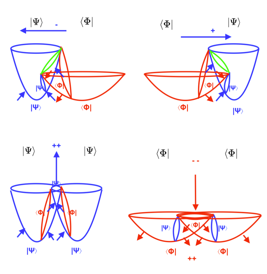
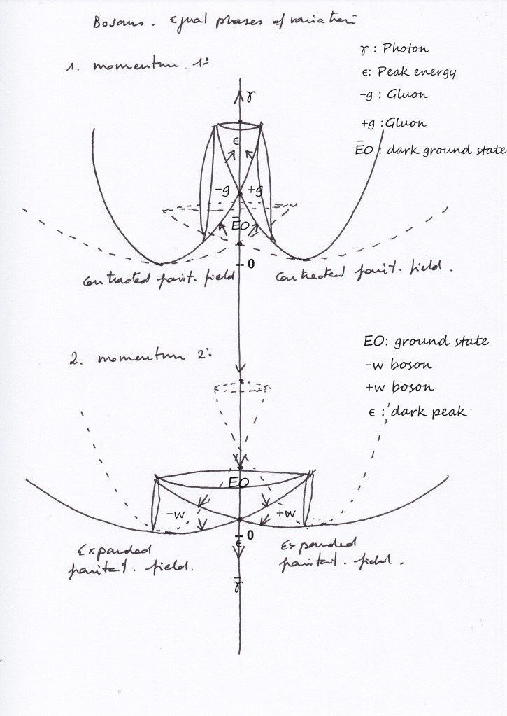
Let us represent it graphically:
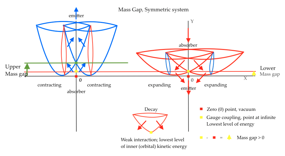
The above graphic represents the bosonic symmetric system; in a similar way it could be represented for the fermionic antisymmetric system, related to the transversal decompressed subfield (for the lower gap) and the transversal compressed subfield (for the upper gap).
The zero point is represented with a yellow point on the above diagram when the intersecting fields expand. The bottom of the descending subfield with the weakest level of density and inner kinetic energy is represented with a black point. An arrow points out the distance between those critical points.
However, in this model the zero point does not represent a vacuum place where no energy and mass exist. The zero point at the moment of the weakest energy in the convex side of the symmetric system is where a double pushing force caused by the positive curvature of the expanding intersecting fields arises. That inverted “dark” pushing force will be equivalent to the force lost by the decaying subfield.
In the antisymmetric system, the lowest energy level occurs when a transversal subfield experiences a double decompression due to the displacement of the negative curvature of the contracting intersecting field and the displacement of the positive curvature of the expanding intersecting field. The corresponding double compression is then experienced by its mirror antisymmetric transversal subfield.
The symmetric and antisymmetric subfields can be described as cobordant subspaces. The vertical subspaces share borders with the left and right transversal subspaces, and they all share borders with the two intersecting spaces.
Those borders can be thought of as the unidimensional line that describes the curvatures of the intersecting fields.
Once this model has been presented in a general way, we will try to describe it in terms of an atomic nucleus using a hypothetical approach as no numerical calculations have been developed for this model yet.
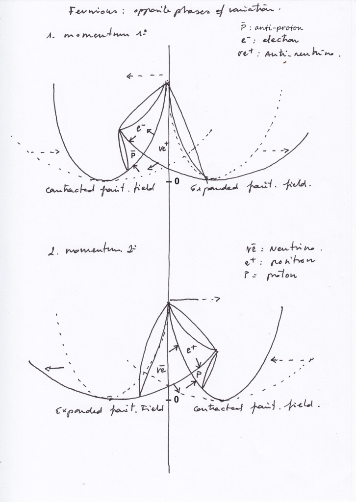
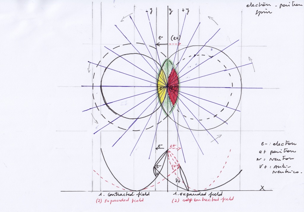
Our atomic antisymmetric nucleus will be formed by a proton, a positron and a neutrino, or by an antiproton, an electron and an antineutrino, depending on the moment we observe the system:
- Antisymmetric system, the left intersecting field expands while the right one contracts:
The right contracting transversal subspace will represent a proton.
The left expanding transversal subspace will represent a neutrino.
The vertical subspace moving towards right will represent a positron.
- Antisymmetric system, the left intersecting field contracts while the right one expands:
The right contracting proton will expand becoming a right expanding antineutrino.
The left expanding neutrino will contract becoming a left-handed contracting antiproton.
The vertical positron will move towards left becoming an electron.
According to that, the right-handed proton will decay into an antineutrino in the right side of the mirror system, while in the left side an antiproton and an electron arise; The left-handed antiproton will decay into a left neutrino while in the right side of the mirror system a proton and a positron arise.
Proton and antiproton, and neutrino and antineutrino, will be Dirac antiparticles at different times; positron and electron, being their own antimatter as they are the same subfield, will be Majorana antiparticles.
In the antisymmetric nucleus, matter and antimatter are mutually exclusive, and their mirror reflections operate at different moments. They are all fermions having a noninteger spin and being ruled by the Pauli Exclusion principle, and they should obey Fermi-Dirac statistics, although this aims to be a causalist and deterministic model.
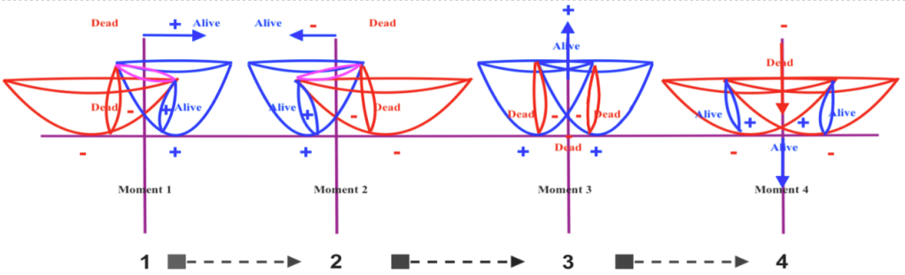
Considering an antisymmetric Schrodinger cat as a figurative example, it could be said that the right alive contracting cat will be the delay reflection of the left dead expanding cat, and vice versa. It can be discussed if they are the future or the passed reflection of each other, but that will only be a way to speak.
Anyways, there will not be a single alive and dead cat, but two identical cats with opposite state and position. And their simultaneous states of being “alive” and “dead” only can be considered “superposed” in the context of their mirror antisymmetry.
It can be visually represented in this way:
The increased or decreased level of energy of the subfields is a scalar magnitude represented by the product of two vectors pointing in the same direction for double compression, or by the division of two vectors pointing in opposite directions for double decompression.
When a parity transformation is applied to the fermionic system, Flipping the signs of all spatial coordinates, all vectors change sign preserving the antisymmetry. Scalars do not change signs, so the term «pseudoscalars» is used in this case.
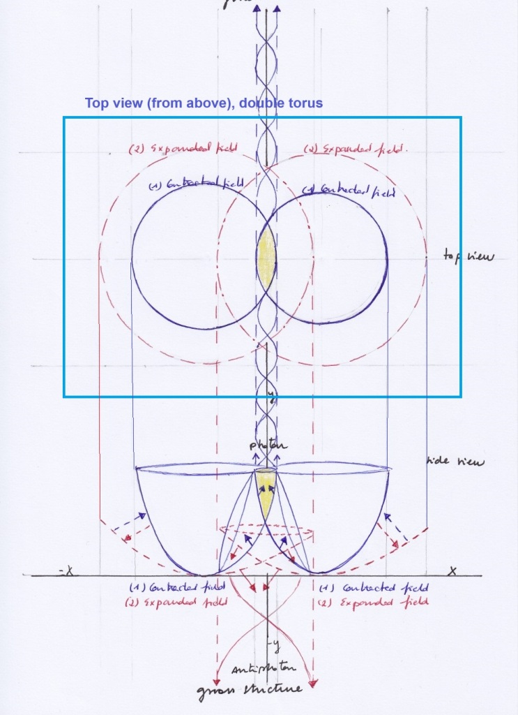
- Symmetric system, when the left and right intersecting fields contract:
The right and left expanding transversal subspaces represent a right positive and a left negative gluon.
The top vertical ascending subspace that contracts receiving a double force of compression will be the electromagnetic subfield that will emit a photon, while pushing upwards.
The inverted bottom vertical subspace at the convex side of the system will represent the dark decay of a previous dark antiphoton .
- Symmetric system, when the left and right intersecting fields expand:
The right and left expanding transversal subspaces may represent -W and +W bosons.
The top vertical descending subspace will be the electromagnetic subfield losing its previous energy, after having emitted a photon.
The bottom vertical subspace at the convex side of the system will be the dark anti electromagnetic subfield that is going to emit a dark anti-photon.
According to that, the left and right transversal subspaces will be mirror symmetric antimatters at the same time. Photon and dark antiphoton will be Dirac antimatter at different times.
But with respect to the bosonic transversal subfields, it seems necessary to have some more clarifications. In this model we are considering two mirror transversal subspaces that are identical reflections of each other at the same present time, i.e., when both intersecting fields contract; a moment later, when the intersecting fields expand, the transversal subfields still will be mirror reflection of each other, but they have been transformed with respect to their previous shape.
In this sense, from the perspective of this model, the transversal subspaces are the same topological subfields that contract when the intersecting fields expand in the weak interaction or expand when the intersecting fields contract in the strong interaction. The strong and weak interactions, then, would be related by the same mechanism. And the mirror transversal subfields that mediate the strong and weak interactions would be the same topological subspaces that are transformed through time.
The model is N=1 because it relates in a supersymmetric way each fermionic subfield with a bosonic subfield.
In that sense, the fermionic electron-positron subfield will be the superpartner of the bosonic vertical subfield that emits the photon when ascending. The fermionic proton-antineutrino subfield, and the fermionic antiproton-neutrino subfields will be the superpartners of the symmetric transversal right and left subfields respectively, when they contract or expand.
The identity of the symmetric transversal subfields, labelled before as W bosons and gluons would require more clarification. Each of those subfields receives a bottom upwards pushing force and a top upwards decompression (in the strong interaction), or a top downwards pushing force and a bottom downward decompression (in the weak interaction).
In the strong interaction, the forces of pressure or decompression of the contracting or expanding intersecting fields will be different, as the contracting fields will have stronger density.
The EM photonic subfield receives a double pushing force from right to left and from left to right caused by the displacement of the negative curvatures of the intersecting fields. Those pushing forces are the same that act decompressing the transversal subfields that expand (labelled as gluons). The emitted photon would have a double helix spin.
Those EM pushing forces are the same that receive the moving right positron and the moving left electron in the antisymmetric system.
On the other hand, the curvatures of the intersecting spaces in this model are gravitational in both the symmetric and the antisymmetric systems. This implies that gravitational fields fluctuate or vibrate. Electromagnetic charges arise from the interaction of those intersecting spaces.
These interacting gravitational fields may be considered as «gauge bosons» in the terminology of field and string theories, while the part where they intersect and form the nuclear subfields could be considered as «gluons.»
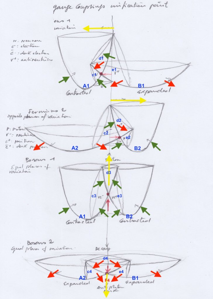
The physical pushing forces created by the displacement of the intersecting fields when contracting or expanding may be interpreted as “quarks”.
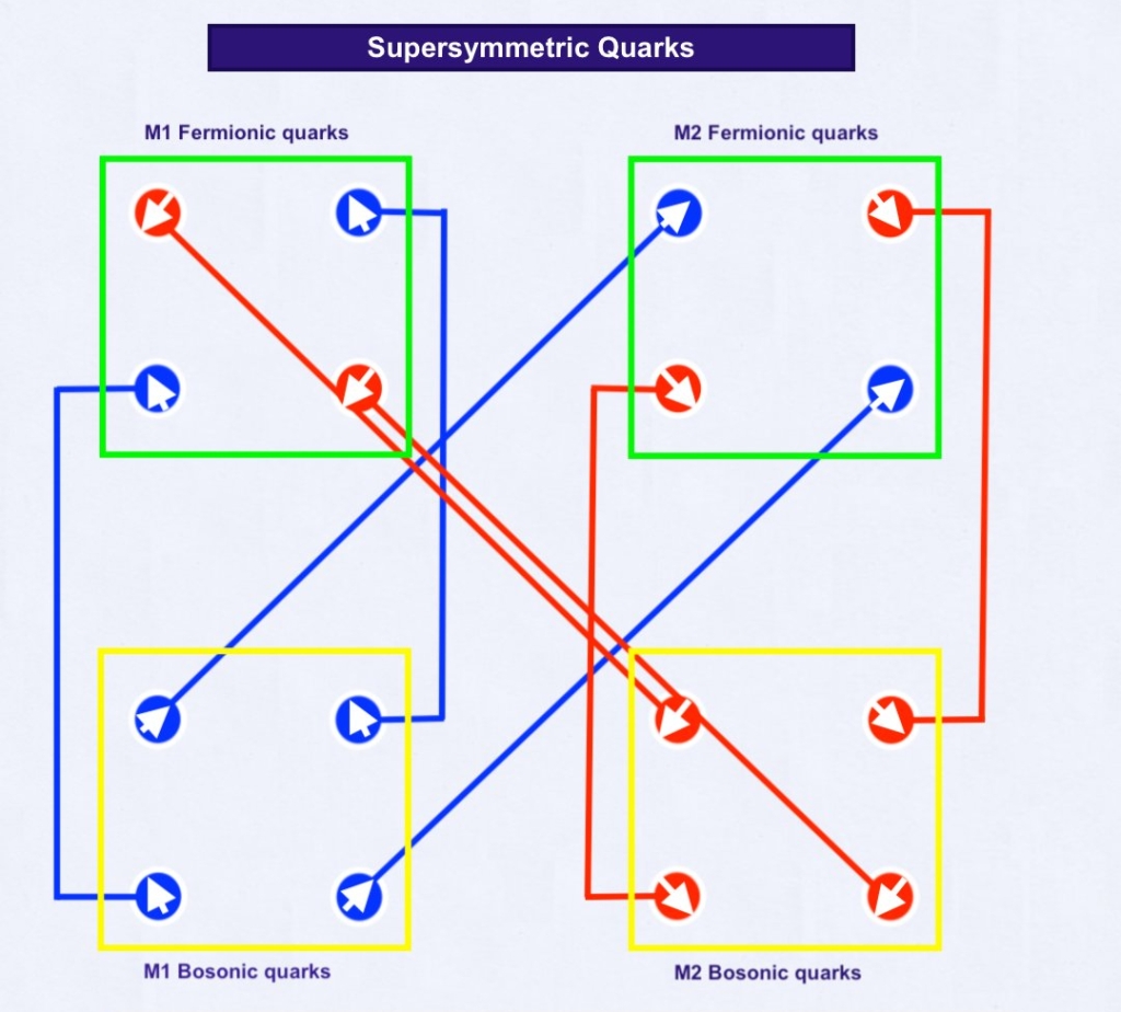
It can be observed that when applying the 90 degrees rotation operator, only two eigenvectors change their sign, and the symmetric system becomes antisymmetric (and vice versa).
These terms would be different ways of referring to the same mechanism. In this sense, it also could be said the supersymmetry of the system would be provided by the way quarks change their sign through time.
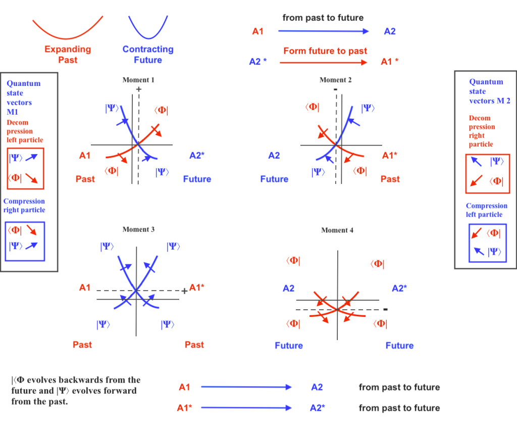
The next diagram shows the way the fermionic and supersymmetric bosonic “quarks” are transformed through time by changing their sign.
The space we have described for the bosonic symmetric and the fermionic antisymmetric systems can be considered as a Minkowski space of 4 coordinates for two different frames of reference: x, y, z, t, for a real frame of reference, and x’, y’, z’, t’, for a complex frame of reference whose coordinates are rotated 45 degrees relative to the real ones.
The 45-degree rotation of the coordinate system implies a partial conjugation that introduces the antisymmetry in the system, as we said before.
A different time dimension for the bosonic and fermionic frames maybe necessary to describe the different dynamics of those systems, either because the subfields have an opposite phase between them, introducing a time delay in their mutual reflection, or because the subfields have an opposite phase with respect to the vibrations of the intersecting fields.
The present model suggests that the bosonic system is also antisymmetric when it comes to the different phases of the transversal subfields with respect to the vertical subfields (which follow the phase of the intersecting fields).
Different mathematical transformations, such as Fourier transforms and Wick rotations, are being used to make antisymmetric systems operationally symmetric.
Mathematical transformations will also be required to relate the two sets of coordinates associated with the fermionic and bosonic systems.
The main difficulty is that the YX coordinates and the diagonal axis that divides the complex plane are referenced by different metrics. A point at Y cannot be rotated to X + iY without increasing the spatial distances.
The same thing happens with the hypotenuse of a right triangle when one tries to measure it with the reference metric of the sides. If the hypotenuse were a rotated side, it would not only be longer than the unrotated sides, but it also could not be precisely determined because of the infinite decimals of irrationality. Two different frames of reference are being measured with the same gauge.
The metric issues between the two reference frames can be managed by adding additional spatial dimensions to separately describe each space-time system or subsystem (in the case of the transversal subfields). However, a type of mathematical transformation is needed to relate the coordinates of the two reference frames. This is the subject of Lorentz transformations in special relativity, which are a type of Möbius transformation.
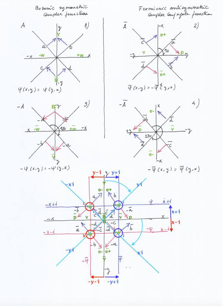
Möbius transformations can be used to project the Y or X coordinates to the X+iY point, virtually removing the complex plane.
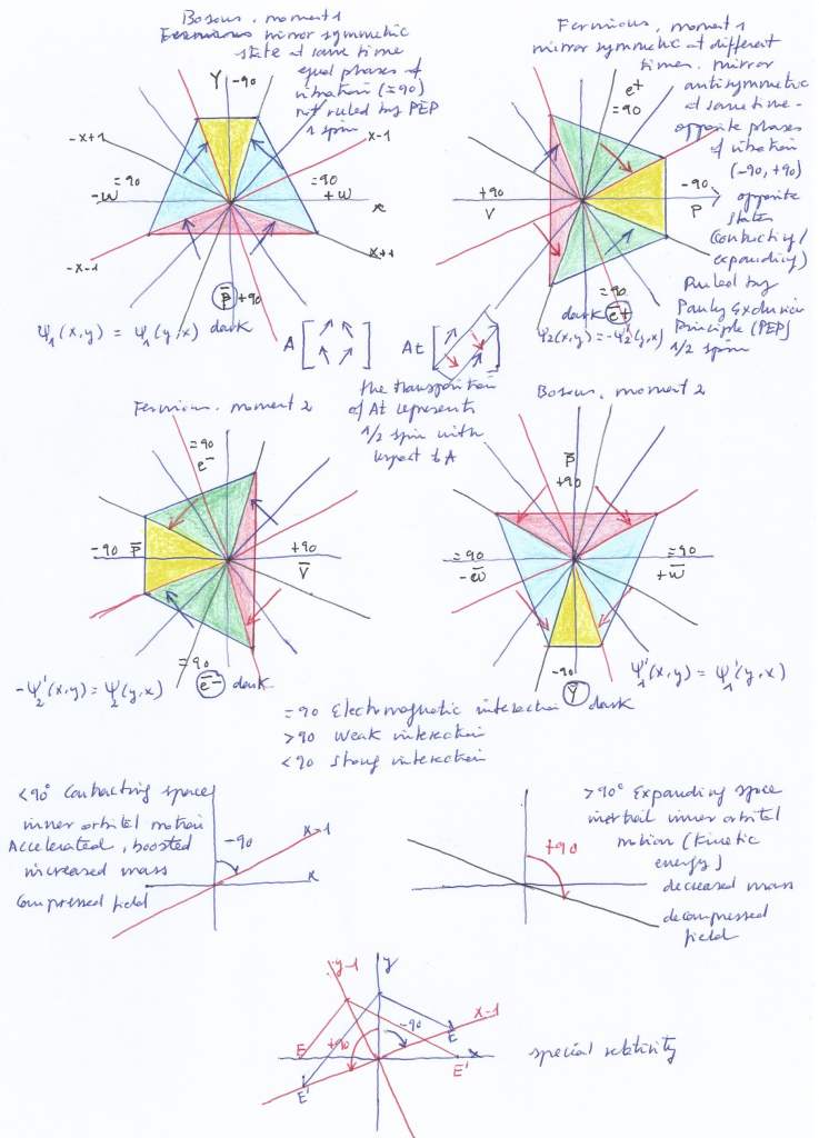
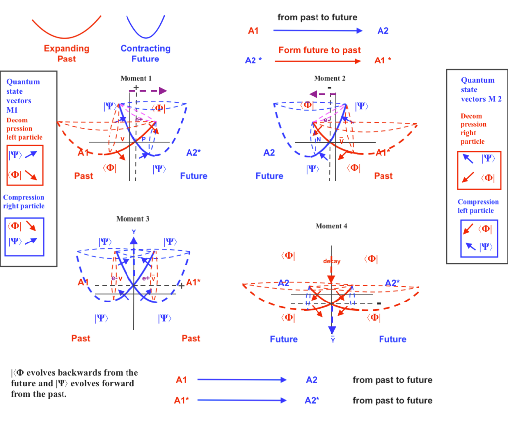
The next picture illustrates the diagram where the eigenvectors of the four transformational 2×2 matrices that combine the bosonic symmetric and the fermionic antisymmetric moments are all superposed as happening simultaneously in the same space.
In the context of operational algebras, in Tomita-Takesaki theory, the change of phase of a half sided modular inclusion can be performed by applying a twist operator, which can be a partial conjugation.
Changing the modular operator, the modular conjugate will be changed in the same degree, creating a different algebraic structure that is not isometric with respect to the untwisted one.
So, changing the modular operator from the A2 matrix to the A3 matrix, the modular conjugate will be A1 (instead of A4). In that way, we can change from the antisymmetric system to the symmetric system and vice versa, in a supersymmetric way, through time.
In Tomita-Takesaki theory, the notion of time is modular. It can be considered as property that emerges or is derived from the dynamics of the modular automorphisms, which represent the evolution of the system over time. In contrast to classical physics, in TT theory time does not exist independently of the system.
Considering time as a real axis tY in the symmetric modular group A1 A3, the partial conjugation operated by a 90 degrees rotation introduces in the system a new time coordinate ti, that is purely imaginary. The sides of the modular operator (and its automorphic modular conjugate) become antisymmetric because the state of half side of the system is going to follow the real time tY, while the state of the mirror side is going to follow the new imaginary time ti, creating a gap time between both sides of the modular operator (and, later, of the automorphic modular conjugate as well).
It’s not only a symbolic formalism, but a mathematical way to describe the dynamics of the rotational system that needs a second time dimension to refer to the harmonic ti phase introduced in the modular group by the partial conjugation.
Commuting the sign of half of the eigenvectors while leaving the other half unchanged implies a partial differentiation that can be interpreted as a fractional derivative, as we saw before. It is that fractional derivation what creates the harmonic or fractional imaginary time and the fractional spins in the modular antisymmetric (anticommutative) group. Fractionality is responsible for the break of symmetry that exhibited the commutative group, introducing anticommutativity.
It is in the context of transforming the commutative modular group into the noncommutative modular group (and vice versa) by means of the partial conjugation given by the rotation that fractionality makes sense. And it’s in that rotational and discontinues frame where Tomita-Takasaki modularity seems to fit.
Considering Δ as the modular operator, J the modular conjugation, and M the intersection of two Von Newmann algebras, Δ^-yt M Δ^it will represent the ½ sided modular inclusions of the modular operator, being t a real time dimension and t’ an imaginary time dimension given by the partial conjugation as we saw before. It is their different time dimension what makes noncommutative, as non-interchangeable, the modular + and – inclusions related to Δ.
Applying the modular involution, we have J^yt M’ J^-it. Δ^-yt is transformed into J^yt and Δ^it is transformed into J^-it’, being J^yt M’ J^-it the involutive automorphism of Δ^-yt M Δ^it. The noncommutative (non interchangable) Δ^-yt and Δ^it become commutative (interchangeable) through time at J^yt M’ J^-it, fixing in that way their antisymmetry.
In the context of our antisymmetric system, we also consider the two vertical subspaces as two modular intersections that are subalgebras of M. Symbolizing the vertical subspaces by ∩, the components of the modular operator Δ that is represented by the matrix A2, can be referred as Δ^-yt M Δ^∩it.
The time evolution given by the modular conjugation will give the mirror symmetric automorphism J^∩yt M’ J^-it. The noncommutative Δ^-yt and Δ^it become commutative through time at J^yt M’ J^-it
The state of contracting or expanding, and the density and inner kinetic energies of the subspaces represented by the modular subalgebras are determined by the vectors of force. But the position of the eigenvectors alone does not determine per se the physical properties of the subfields which they are related to.
The eigenvectors serve as a symbolic representation of the pressure forces caused by the intersecting fields during expansion or contraction, determining the curvature, shape, density, and internal kinetic energy of the subfields and their associated time.
The eigenvectors’ direction, when it comes to the 90-degrees rotated symmetric system of intersecting fields that simultaneously contract, is going to be identical to the direction they would have in an unrotated antisymmetric system of two intersecting fields vibrating with opposite phases, when the left field expands while the right one expands.
The eigenvectors can be thought of as the complex variables of a biholomorphic function formed by a complex and a conjugate function that are mutually interdependent. Their fractional differentiation given by the fractional conjugation that occurs when applying each 90 degrees rotation is visually represented by the matrix’s modularity.
The constructive interrelation of the complex and conjugate functions represented by the mentioned complex A1,A3 and conjugate A2,A4 matrices respectively can be interpreted as well as Bäcklund transformations, where the conjugate function transforms the complex function and vice versa. The prototypical example of a Bäcklund transform [4] is the Cauchy-Reimann system, where “a Bäcklund transformation of a harmonic function is just a conjugate harmonic function”.
In the context of representation theory, we may also interpret the antisymmetric system of subspaces represented by the matrix A2 as an original vector space, and its negative mirror reflection matrix A4 as a dual vector space. To connect A2 and A4, forming their isometric automorphism through time, it’s necessary to pass through A1 (the identity matrix) and A3 by means of the fractional differentiation or partial conjugation given by the transformation matrices when applying the 90 degrees rotational operator.
The bridge that fixes the gap between A2 and A4 will be related to the Langlands parametrization. The Langlands dual group that allows the creation of the automorphism between the subspaces of the antisymmetric system will be represented by the conjugate matrices A2 (90º) and A4 (270º), and the complex matrices A1 (0º) and A3 (180º).
The two eigenvectors that determine the curvature of each transversal subspace and the sign commutation of ½ of each pair that causes the transformations of the system would be related to Cartan-Killing pairing.
Additionally, considering as an example the antisymmetric system where the left transversal subspace L contracts at t1 while the right transversal subspace R expands at t2, and the left transversal subspace expands at t1’ while the right one contracts at t2’, it can be suggested that the expanding Lt1’ will be the functional Galois extension of Lt1, and Rt2 will be the functional Galois extension of Rt2’, connecting the intersecting fields model as well with the Langlands program.
The collection of 2×2 complex matrices may also be related to Bethe transfer matrices [5] of eigenvectors related to complex and conjugate functions in the context of quantum integrable systems.
The unit circle mentioned at the beginning may be interpreted as a flattened version of the unit sphere, which is a visual way of representing geometrically the rotations of nuclear spins in ½ particles. That unit sphere is also related to Bloch theory. [6]
In the model introduced by this paper, nuclear rotation seems necessary to quantize the classical system of intersecting fields, causing the apparent discontinuity that breaks symmetry and antisymmetry, giving place to modularity.
With respect to modularity, the introduced model can be described in terms of moduli spaces of a Higgs bundle. Higgs bundles were introduced by Nigel Hitchin. In the present model, the two intersecting fields would represent a Riemann geometry system. The vertical subspace (and its mirror inverted counterpart) would represent the Higgs field that mediates between the left and right transversal subspaces, giving them their masses.
Both the left and right transversal subspaces, together with the intermediate Higgs field, form the moduli space of Higgs bundles. The transversal subspaces represent the boundary components of the moduli space, while the Higgs field acts as a bridge between them.
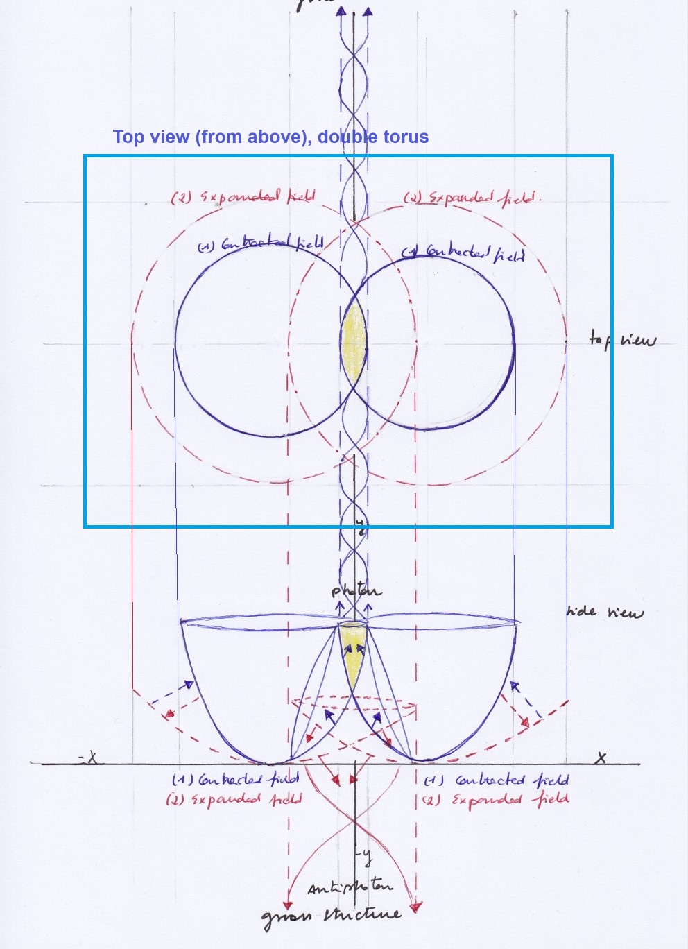
Those boundary components are frequently represented by two transversal tori. As we will see later, we interpret the torus’ inner curvature as a contracting transversal subspace and the torus’ outer curvature as the expansion of that transversal subspace.
The next figure [7] represents a Moduli space of Higgs bundles: The left and right tori on the linked figure represent the Higgs bundles, the central circles in red represent the Higgs field, and the blue curved would represent a Riemann space: https://link.springer.com/article/10.1365/s13291-021-00229-1#Fig5
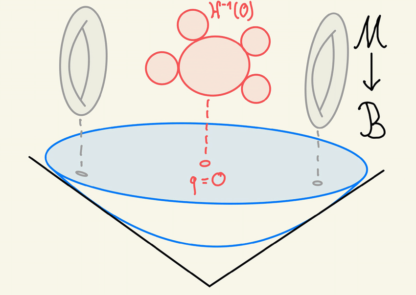
The above figure, the tori have non chiral symmetry. Having both transversal subspaces chiral mirror symmetry, and considering the transversal tori’s curvatures as the simultaneous representation of the two states (contracting or expanding) of transversal subspaces that are symbolized by the tori, this interpretation allows us to relate the inner and outer curvature of both tori to form mirror symmetric or antisymmetric relations, as we have seen before.
In our model, the Riemann space is not a single curved space but two intersecting spaces.
It is not clear enough in this paper if the rotation of the whole system would actually transform per se the physical properties and phase times of the subfields, or if their periodic synchronization and desynchronization would require an additional explanation. Misinterpreting the physical meaning of the symbolic formalism given by the eigenvectors’ directions seems a possibility in this model.
To conclude, we can relate the atomic model to other theories and developments, using a visual approach as well.
In the context of string theories, the border of the positive and negative curvatures of the intersecting fields, or of parts of them, may be saw as one-dimensional strings:
Another way of visually considering the symmetric and antisymmetric systems from a strings perspective could be this:
As well in the context of string theories, the intersecting fields that interact to form the nucleus of subfields may be related to the positive curvature of de Sitter vacuum spaces, when expand causing an outward pushing force, or to the negative curvature of anti de Sitter vacuum spaces [8], when they contract causing an inward pushing force.
The symmetric and antisymmetric systems may also be related to the Ramond-Ramond or the Kalb-Ramond fields [9]. The Ramond-Ramond fields are antisymmetric tensor fields with two spacetime indices, which is a mathematical way to refer to two fields in a dual system.
The transversal subfields of the symmetric and antisymmetric manifolds could be related in some ways to Calabi-Yau transversal spaces. Calabi-Yau however demands smaller sizes for the spatial higher dimensions and a compactification.
We can visually relate the elliptic orbits inside of the transversal subfields, caused by their periodical expansion and contraction, and relate them to the notion of elliptic fibrations used in String theories:
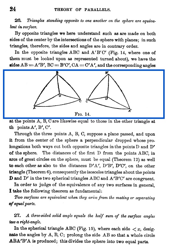
The shape of the nuclear transversal subfields, on the symmetric or antisymmetric diagrams, reminds the shapes drawn by Lobachevsky when explaining his imaginary geometry (2).
Note that the inner curvature of the transversal subfields is half concave and half convex: their concave or negative region curves inwards, and its convex region curves outwards.
Quantum mechanics, field and string theories have been developed mainly as abstract mathematical models with no visual spatial references.
However, tori geometry is generally used in different ways by many theories to aid visualization and simplify calculations.
The intersecting spaces can also be thought of as intersecting tori. The outer positive and the inner negative curvatures of the torus will be the simultaneous representation of the expanding or contracting moments of a vibrating field when looking at it from above in an orthographic projection.
Double genus geometry is being used in the context of diatomic molecules. However, the notion of a single atom as a dual structure with a shared nucleus, is not being considered by mainstream physics. A theory that can be close to the intersecting fields model is the multiverses theory, as the intersecting spaces may be interpreted as parallel universes that interact by means of their mutual intersection to form a composite manifold of vertical and transversal parallel sub universes.
The presented model can also be expressed in terms of emitter-absorber transactional models that correlate advanced and retarded waves, taking place a transactional “handshaking” between them when interchanging energy. In that context there are some similarities as well with the reflection positivity property that we saw before.
Many different and abstract approaches from diverse mathematical branches, developments and tools seem to be considering same or very similar physical structures in unrelated ways. In this sense, we can also mention the vertex operators’ formalism, where fields are inserted at specific locations of a two-dimensional space. In our model, the vertex point would be given by the intersecting of the generating fields. It would also represent the coupling gauge point in the present model.
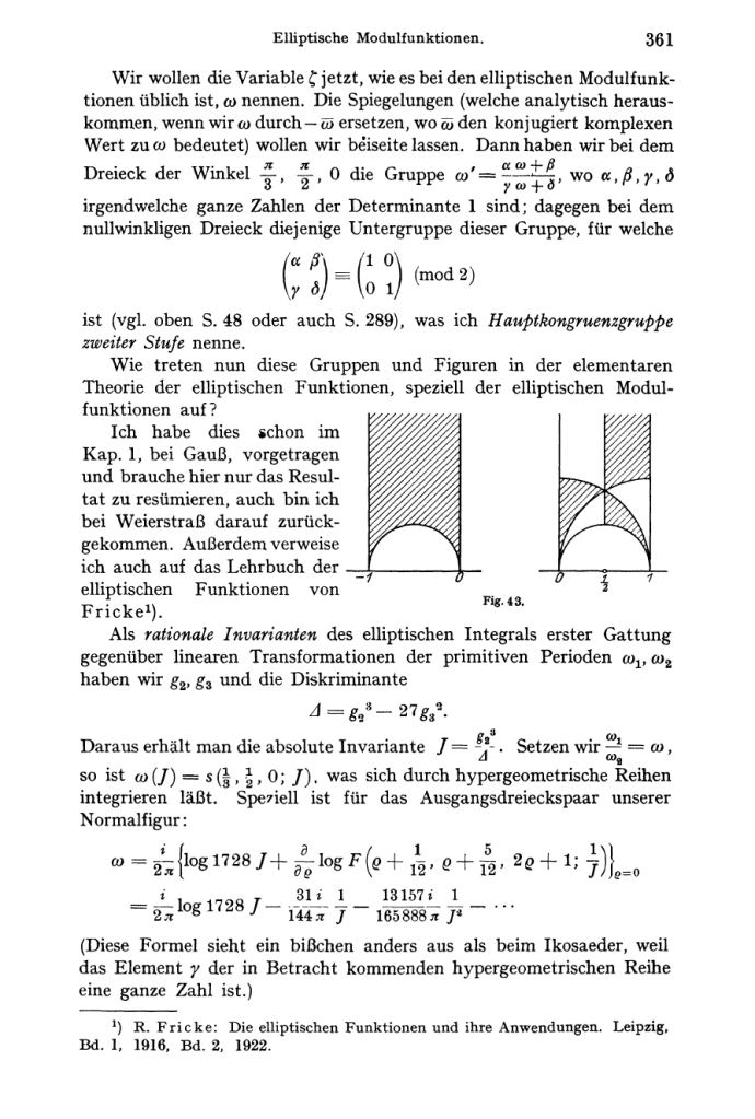
On the other hand, it can be interesting to mention thar “a significant role in Klein’s research” – when he developed the geometric theory of automorphic functions combining Galois and Riemann ideas – “was played by pictures” related to “transformation groups (linear fractional transformations of a complex variable)”. [11]
The Klein’s drawing related to elliptic modular functions is the same two-dimensional figure that forms the cobordant nucleus in the intersecting fields models, showing the half convex and half concave transversal subspaces, the double concave curvature of the top vertical subspace and the double convex curvature of the bottom vertical curvature. [12]
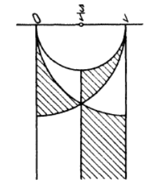
The above picture shows the Klein’s drawing rotated. The below picture shows it in its original form:
The fields and subfields of the model can also be interpreted as fluctuating vortices. Some quantum theories, as Chern-Simons theory, consider vortices instead of fields.
The article, “The Chern-Simons current in systems of DNA-RNA transcriptions” [13], provides an interesting image about a loop space as Hopf fibration [14] over DNA molecule [15], that seems similar to the diagrams about elliptic fibrations of the transversal subfields previously presented.
The original aim of the present research was to find the mechanical flaw that drives anomalous cell division, assuming there must be a mechanism where the processes occur with a normal path, and an acceleration or deceleration of those processes will cause gene anomalies.
Considering a cell as a dual system, some similarities must exist with the dual model we have presented.
A fundamental role during cell division is played by the rotation of the spindle axis. And it’s known that abnormal spindle rotation [16] can result in genetic abnormalities.
We hope the presented fields model may provide some additional clues about modulating anomalous cell division and differentiation.
Additional diagrams:
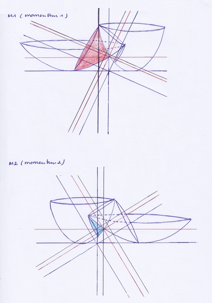
Image 1/7. Frames of reference, antisymmetric system
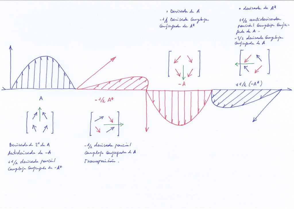
Image 2/7. Fermionic and bosonic representation
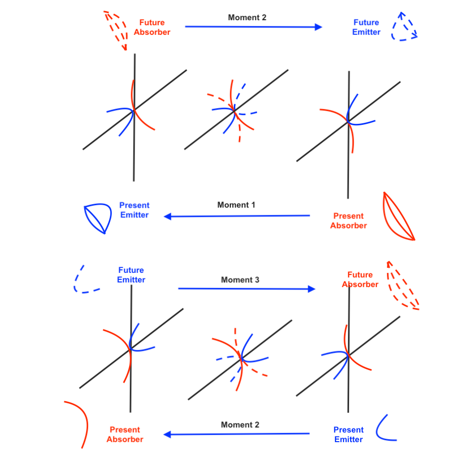
Image 3/7. Transactional interpretation
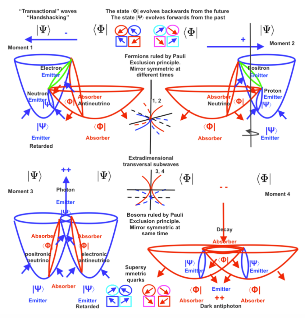
Image 4/7. Handshaking, transactional interpretation
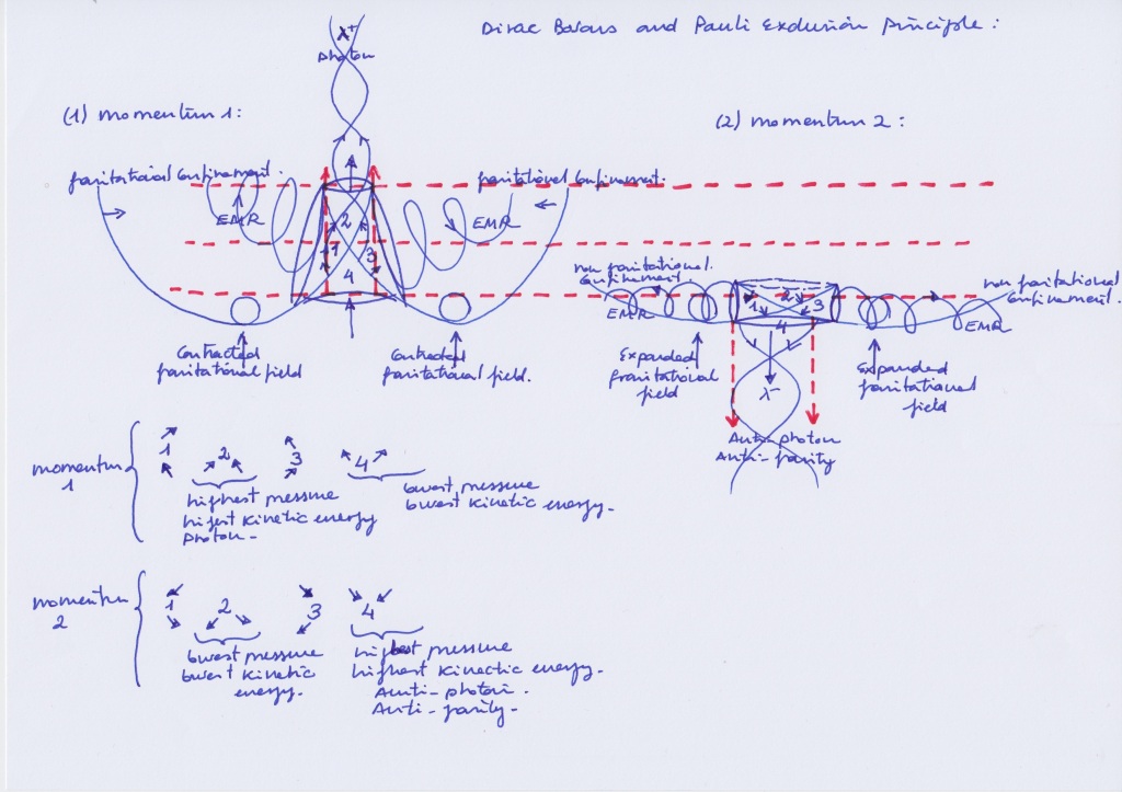
Image 5/7. Symmetric system
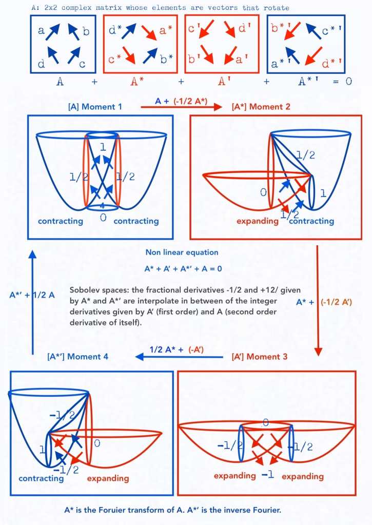
Image 6/7 Fourier transform. Fourier inverse
References
[1] Supersymmetric Yang Mills theory (SYM): https://en.wikipedia.org/wiki/N_%3D_1_supersymmetric_Yang%E2%80%93Mills_theory
[2] Sobolev interpolation: https://en.wikipedia.org/wiki/Interpolation_space
[3] Convolution; Reflection positivity: https://www.arthurjaffe.com/Assets/pdf/PictureLanguage.pdf
[4] Bäcklund transform: https://en.wikipedia.org/wiki/B%C3%A4cklund_transform
[5] Bethe matrices: https://arxiv.org/abs/math/0605015
[6] Bloch sphere: reference request – First occurrence of the Bloch sphere in the scientific literature – History of Science and Mathematics Stack Exchange
[7] Moduli space of Higgs bundle, Fig, 5: The left and right tori on the linked figure represent the Higgs bundles, the central circles in red represent the Higgs field, and the blue curved would represent a Riemann space): https://link.springer.com/article/10.1365/s13291-021-00229-1#Fig5
[8] Anti de Sitter space: https://en.wikipedia.org/wiki/Anti-de_Sitter_space
[9] Ramond-Ramond fields: https://en.wikipedia.org/wiki/Ramond%E2%80%93Ramond_field
[10] N. Lobachevsky: “Geometrical Researches on the Theory of Parallels” (pág 24) https://www.google.es/books/edition/Geometrical_Researches_on_the_Theory_of/GJBsAAAAMAAJ?hl=en&gbpv=1&pg=PA22&printsec=frontcover
[11] “Geometries, Groups, and Algebras in the Nineteenth Century” by I. M. Yaglom, pág. 130.
[12] F. Klein, “Vorlesungen über die Entwicklung der Mathematik im 19. Jahrundert”, pág. 361
[14] https://en.wikipedia.org/wiki/Hopf_fibration
[16] https://en.wikipedia.org/wiki/Spindle_apparatus
An updated version of this article can be downloaded here:
